When Simple Measures Fail: Characterising Social Networks Using Simulation
Bruce Edmonds (Centre for Policy Modelling, Manchester Metropolitan University) and Edmund Chattoe (Department of Sociology, University of Oxford)
Abstract
Simple egocentric measures are often used to give an indication of node importance in networks, for example counting the number of arcs at a node. However these (and even less obviously egocentric measures like centrality and the identification of cliques) are potentially fallible since any such measure is only a proxy for the structural properties of the network as a whole. The effectiveness of such proxies relies on assumptions about the generative processes which give rise to particular networks and these assumptions are not (and possibly cannot be) tested within the normal framework of Social Network Analysis (SNA). In case studies of real social networks it is often difficult to get enough data to evaluate how faithfully the standard network measures do characterise the network. Given these empirical and methodological difficulties, therefore, we use a set of agent-based simulations as case studies to investigate some of the circumstances in which simple measures fail to characterise key aspects of social networks. Using this approach we start to map out situations where simple measures might not be trusted. In such circumstances, we suggest that an alternative approach (in which agent-based simulations are used as a sort of dynamic description capturing qualitative facts about the target domain) might be more productive.
Introduction
Looking at the process of “normal science” in SNA suggests a potential concern with measurement. In traditional (typically linear) statistical models, the measured “variables” serve as inputs to the modelling process, with the corresponding model coefficients forming the “outputs”. These coefficients tell us what the patterns of association are between variables (however these are defined). Notoriously, even when a coefficient is significant, it does not explain the observed association but can only measure it. Thus it is necessary for further research to hypothesise how a particular association comes about: what the causal mechanism is by which the observed association arises (Hedström and Swedberg 1998). If the relevant causal factors can be measured quantitatively and the mechanism is one that can be captured in a statistical model, quantitative methods can again be used to show that the corresponding mechanism is at least not disproved. In the case of social network analysis, however, matters are more problematic on two counts. Firstly, the “measures” of network properties (corresponding to variables in linear statistical models) may be attempting to approximate properties of the whole network, a task for which they are more or less well suited. The most individualistic measures (like density) are most likely not to capture the overall “flavour” of networks but even for obviously structural measures like centrality and cliques, we are still entitled to ask how well these “sub network” measures should be expected to capture properties of the whole network. Secondly, and following from this, the kinds of explanations that can (and should) be used to account for observed associations between characterisations of networks unfortunately depend on the properties of whole networks. This is what we mean, in the limit, by a “structural” approach to social understanding.[1]
Thus, when we say that tie density in an information network is associated with success in the job market, we have more to worry about than we do when we say that education level is associated with lower divorce risk. Firstly, it is always possible that the explanation of a traditional statistical association is direct. Perhaps something learnt progressively in education (like the ability to understand competing points of view) actually reduces the risk of divorce on an individual basis. SNA cannot readily offer these direct explanations because the whole basis of the network approach is that information, reputation, favours and other “resources” are transmitted in a complicated way that means they end up allocated differentially to actors in the system. Secondly, even if they are not direct, the statistical approach seems to require its explanations to be rather simple in practice (Abbott 2001). By contrast, the explanations available in networks can depend (in the worst case) on their precise architecture, such that no characterisation of any sub networks or their associations is an adequate representation to explain the observed outcome. This is what is meant by a complex system and is captured in the notion of algorithmic compressibility. Some systems (like a linear relationship in physics) can be captured by algorithms that are clearly much “simpler” or “more economical” than the systems themselves (in this case, an equation of the form y=ax+b). By contrast, the most economical representations of certain systems are the systems themselves.
This insight should not be overplayed. It is possible, indeed likely, that the normal scientific process has established at least some SNA measures which do, in fact, well characterise the networks to which they are applied (at least in some cases). It may also turn out that social networks are not complex in this worrying way. This paper is therefore concerned with a slightly different question: how might we tell whether or not there is a problem of this kind and how much of a problem is there? We advocate agent-based simulation to address this question on two grounds, associated with the two concerns already raised.[2] Firstly, empirical network studies are often (of necessity) quite small and this means it is hard to use the resulting data for exploration of alternative measurement strategies. Even if there is sufficient data for this task the other problem (that of explanation) rears its head. One cannot judge alternative characterisations of a network solely in terms of the quality of the associations they provide since these associations must be explained before they can be evaluated as genuine rather than merely spurious. Traditional SNA, like traditional statistics, does not have the tools at its disposal to explore the ramifications of proposed causal mechanisms unless they are very simple or direct. By contrast, agent based simulation involves specifying both a set of individual behaviours/attributes and unfolding the dynamics of social interactions to include the evolution of networks. This means that we can both measure simulated networks in different ways (just as we can real networks but on a much larger scale) but also (as we typically cannot do with real networks) investigate whether the network characteristics we choose to measure correspond effectively to the causal mechanism proposed. For example, suppose that we wanted to explain an association between how many ties a node has and how soon it hears some “gossip”. Clearly, if the mechanism of gossip is that everyone who hears it immediately tells everyone they know it is hard to see how number of ties would not have a robust and explanatory association with how soon one hears. If, however, the social rules of gossip are more complex, it becomes much harder to be confident that a “tie count” will yield a measure that is strongly explanatory rather than simply weakly associative.
There is another issue to consider in the context of network measurement and that is the role of dynamics. In most SNA, the task is to reconstruct a static network. Even in “dynamic” studies, what is actually created is a set of static networks at fixed intervals (Barnett 2001). SNA is well aware that any static network is a “snap shot” of a truly dynamic process in which individuals interact and change both their attributes (wealth, attitude and so on) and network positions.[3] The question is then what we assume about the effective characterisation of a dynamic network from a static “snap shot”. At one extreme, it is possible that the underlying generative mechanisms maintain certain characteristics of nodes so a well-connected node at period 1 is also well connected at period 2. On the other hand, in the worst case, even the distribution of a characteristic over the population of nodes may not remain stable as the network evolves. Under these circumstances, associations between network measures may or may not capture the underlying generative mechanism. At worst, an apparent association at a particular time point may simply be an artefact of the current state of the network which would not be found if the network was measured one period earlier or later or earlier. (The difficulties of conducting empirical SNA mean that this problem is rather unlikely to be detected.)
The case studies offered in the next section illustrate how simulation can be used to explore these issues and offer some illustrations of the potential weaknesses of simple network measures.
Some Simulation Case Studies
In this section we apply the same “thought experiment” to a set of diverse social simulations involving networks: imagine that the model accurately represented the social phenomena one was investigating – to what extent would egocentric measures be a good characterisation of the role that nodes were playing in the system?[4]
The P2P Model
This is a model of nodes in a peer-to-peer (P2P) network. A P2P network is a computer-mediated network that uses the Internet for file sharing and searching. Such networks are of wider social interest because they can be developed to represent such phenomena as the creation of social capital in communities through the exchange of favours.
In this simulation, nodes seek files by sending queries through the network using a “flood fill” algorithm – contacting everyone they know – for a set number of “hops” (arc transitions).[5] This is a decentralised network in that each node only “knows” about a limited number of other nodes and is not aware of the whole network (for example via access to a central server). To search the network a node sends its query to the nodes it knows and they pass it on to those they know and so on. This process continues until the queries have been passed on for a certain maximum number of hops at which point the relevant copy of the query “dies”.
If a node is currently sharing its files (it does not have to) and it happens to possess a requested file, that file is sent back to the originator of the query. Each node has a “satisfaction” level. When a node gets a file it does not have (and wants) its satisfaction level increases. Satisfaction decays exponentially at 10% per cycle. This means that nodes have to keep succeeding in their quest for files if they are to remain satisfied. If the satisfaction level of a node drops low enough then it will copy the connections and sharing strategy of a neighbouring node which is doing better (or with a low probability drop out of the network altogether and be replaced by a new node with a single random connection). This constitutes a social imitation process based on relative performance.
The network is directed so that if node A sends queries to node B the reverse does not necessarily occur.[6] Each node thus represents a person who is controlling some P2P software on the Internet. If the controller is unsatisfied with the number of files they are getting they may choose to imitate the way that another controller operates their software.
The general structure of the network that develops is illustrated in Figure 1 below. Due to the dynamics of the model a core partition develops which is totally connected and the rest of the network (the periphery) mostly consists of branches that link into this core either directly or indirectly. There may also be one or more small isolated groups which quickly “die”. This is a result of the dynamic node behaviour. If there were any nodes that were on a branch leading away from the core, these would not be viable in terms of file searching success and hence their satisfaction level would fall until they reset their connections to random ones thus “breaking” the branch. Of course, before this structure is established (and during transitory periods afterwards) different patterns may occur but the combination of core partition and periphery is the “attractor” for the system.
Figure 1. An illustration of the typical network structure that results in the P2P model – there is a core partition that is totally connected and a collection of branches feeding into this. Arrows show the directions in which queries for files might be sent.
The particular simulation that forms the basis of this case study is composed of a population of 50 nodes simulated over 1000 time cycles. Unless otherwise stated, the statistics quoted are from the last 600 time cycles to allow time for the simulation to settle down into some sort of dynamic equilibrium.
The core is usually totally connected and formed of an overall minority of the nodes but typically dominates any other totally connected partitions in the system. Figure 2 shows the sizes of the partitions during a typical simulation run. Usually the dominant partition consists of between 3 and 20 nodes whilst the other partitions involve 2-5 nodes.
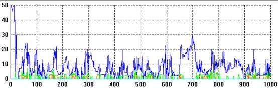
Figure 2. The distribution of sizes for totally connected partitions in the simulation. The size of the largest at any time is shown in blue, the next in green, followed by orange, red and so on.
In this simulation, the number of nodes that decide to share their files quickly increases to between 40% and 90% of the total.
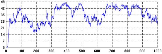
Figure 3. The number of nodes sharing files over time.
We will consider four types of node: those in the core that share (in-coop), those in the core that don’t share (in-def), those in the periphery that share (out-coop) and those in the periphery that don’t share (out-def).
Whether the node is in the core partition and whether it is sharing its files both have an impact on the extent to which two measures of centrality are correlated with its satisfaction level. One would expect that the centrality of a node (assessed both by the number of outward links it had and by the corresponding Bonacich[7] measure of centrality) would be correlated with the level of satisfaction, since having access to more nodes should make querying more productive. This is true but to a varying and minor extent. Table 1 shows Pearson correlation coefficients with the dependent variable being the node satisfaction level for different types of nodes and the independent variables being the number of links, the number of links 6 cycles ago, the centrality and the centrality 6 cycles ago.
Table 1. Pearson correlation coefficients with current node utility for 4 types of node
|
Type |
Number of links |
Number of links lagged 6 periods |
Centrality |
Centrality lagged 6 periods |
|
in-coop |
-0.058 |
0.13 |
-0.062 |
0.12 |
|
out-coop |
0.073 |
0.17 |
0.065 |
0.16 |
|
in-def |
0.039 |
0.074 |
0.067 |
0.087 |
|
out-def |
-0.15 |
-0.053 |
0.066 |
0.13 |
There are a number of things to note about these results. Firstly, that none of the measures explains more than 17% of the node satisfaction. A lag of 6 cycles turned out to give the maximum correlation. (Figure 4 shows the correlation between number of links and centrality for different lags. This shows that the poor result is not simply a side effect of inappropriately chosen lags.)
Figure 4. The correlation between two centrality measures and satisfaction level for different lags (over all types of node).
Secondly, with the notable exception of the number of links for out-def, the correlation for a lag of 6 is higher than it is with no lags. This is not surprising since it takes a number of cycles for a query to propagate down the network and for the files to be returned which will only then increase the satisfaction level. The exception to this pattern is that the number of links for out-def nodes has a stronger (negative) correlation with no lag than with a lag of 6 cycles. This occurs because the lack of links for a node sometimes results from its previous higher satisfaction level. What sometimes happens is that a node in the core partition is (or becomes) a non-sharer. This reduces the satisfaction of the other nodes in the partition because they bear the cost of its queries but gain no files from it. This makes it slightly more likely that they will re-organise themselves and effectively exclude the non-sharer, leaving it on the periphery (or isolated) and hence without present links.
Thirdly, the correlation is sometimes very different for the different types of node. For example whilst the correlation for out-coop nodes is just above the 15% level, that for in-def nodes is much smaller. The fact that there are significant differences between the types of nodes is reinforced by the differences in the averages for satisfaction level, number of links and centrality for the four types shown in Figure 4.
Table 2. Average network properties by node type: Network connections
|
Type |
Average utility |
Average number of links |
Average centrality |
|
in-coop |
0.790694 |
2.967343 |
0.405458 |
|
out-coop |
0.512293 |
2.500713 |
0.309861 |
|
in-def |
0.373527 |
2.005525 |
0.269064 |
|
out-def |
0.324489 |
1.492763 |
0.189887 |
It is interesting to compare this case with a variant of the model in which the only thing that is changed is that when a query is to be sent down a link, it is sent to a randomly chosen node (effectively cancelling the network structure). Thus, in this version, if a node has 3 outward links, it will send queries to 3 other randomly determined nodes. The average network properties for this version of the simulation is shown in Table 3. They are remarkably similar to those from the non-randomised model, except that the in-def nodes achieve a higher satisfaction and centrality. This occurs because their satisfaction will not be “dragged down” by nodes that imitate them and hence use the same connections and negative share strategy. This strategy is not available when the connections are randomised.
Table 3. Average network properties by node type: Randomised connections
|
Type |
Average utility |
Average number of links |
Average centrality |
|
in-coop |
0.707675 |
3.062462 |
0.409185 |
|
out-coop |
0.51401 |
2.688987 |
0.320872 |
|
in-def |
0.504822 |
2.62037 |
0.353121 |
|
out-def |
0.313881 |
1.881392 |
0.224612 |
To give a better flavour of the dynamics at work in this simulation, we will trace some of the history of a single node. Some node statistics are shown in Figure 5 which charts the number of outward links the node has, its centrality, its satisfaction level and whether it is currently sharing its files or not.
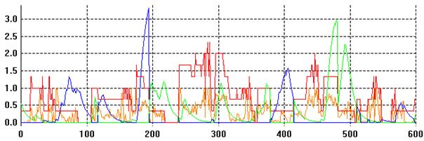
Figure 5. The last 600 cycles of a simulation run for one particular node. The red line shows 1/3 of the number of outward links the node has. The orange line shows the measure of centrality: from 0 to 1 with 1 being the most central node. The blue/green line shows the level of satisfaction for the node. (It is blue when it is not making its files available for sharing and green when it is.)
A detailed history of the node (although unfortunately not obvious from the above graph) can be gained by a detailed inspection of its state and the overall network structure. (Times will be given using the scale in Figure 5.) At cycle 50 the node is in the mid periphery region, with only one outward link but via that link it reaches a large number of other nodes (hence the high centrality). It is not sharing its files. By cycle 75 it has found several of the files that it was looking for and thus has an increased satisfaction level. However, this has lowered the satisfaction of other nodes around it and so these have ceased to link to it and it has thus become a leaf node on the edge of the periphery. Next the node it links to resets (due to its low level of satisfaction) and the inspected node becomes isolated. Because of this isolation it eventually resets itself (twice). At cycle 180 the inspected node is just outside the core with many links into it. Since the core is presently composed of many file sharers, the inspected node is doing well at this point.
In contrast, Figure 6 is a scatter graph for this node illustrating the absence of an overall strong correlation between the number of outward links and its level of satisfaction.
Figure 6. A scatter graph for the number of outward links from the inspected node (lagged by 6 cycles) against satisfaction level recorded between 400 and 1000 cycles.
It is clear that, in this model, it is important to distinguish the effect of node centrality with respect to both the kind of node (sharing or otherwise) and to its position in the overall network structure (periphery or core). Simple uniformly applied centrality measures prove not to be very helpful in this case.
At this point, it will be useful to revisit the arguments presented earlier in the light of this case study and try to address some potential criticisms of this approach. Firstly, it might be argued that this simulation either isn’t very realistic or, if it is realistic, it only accurately represents a mechanical rather than a social process. This may be true, although it should be clear that the P2P model could easily be made much more social.[8] However, it is not clear that this criticism justifies disregarding a concern about the effectiveness of SNA measures. In the first place, we are in a position to show that these issues arise in a number of different simulations with varying degrees of sociality. In the second, we could easily develop this model in a more social direction and see whether the same results obtained. A second criticism is that we are setting up a “straw man” and that node densities (and even centrality) are very basic measures of network structure. If this network were “properly” analysed by SNA, the critics might claim, the most effective network measures would have been applied based on study of the system. This criticism can be tackled in three ways. Firstly, we can observe the kinds of SNA that are typically done to see how commonly such simple measures are applied in practice. Secondly, we can investigate more sophisticated measures using the same simulation although there wasn’t time to do that for this conference. Thirdly, we can challenge the critics about being “wise after the event”. Of course, once the generative mechanism has been laid out and analysed in simulation it is possible to see that sharing status and core/periphery position will be crucial determinants of satisfaction not captured by numbers of outward ties. However, a typical piece of SNA does not have this access to the generative mechanism. Instead, it has a more or less accurate “snap shot” of the network and (much more rarely) some qualitative data about individual behaviour. The reader will have to judge, from their own experience, whether it is likely that SNA would “hit on” the correct generative mechanism, given the typical analysis it would apply to the file sharing domain.
Subject to these concerns, the results of the simulation provisionally appear to support the initial concern with measurement. Network density and centrality do not, in this case, explain very much about node satisfaction levels and it is only simulation that allows us to say much about why this is so. Interestingly, however, randomising the network doesn’t explain much less about the system suggesting that what matters in this particular model (to the extent it matters at all) are properties like the average number of ties rather than their precise arrangement. The ability to randomise a network in this way suggests an important advantage of the simulation approach in identifying genuinely complex networks, those in which the randomised network behaves very differently from the non-randomised one.
An Extended Schelling Segregation Model
We now turn to a second (and substantially different) example to get a sense of whether the first result was somehow untypical. In this case, the social network is fixed at the start of the simulation based on a number of parameters. These parameters are the number of friends for each node, the degree to which friends are selected from the same initial locality and the degree to which friendship choice is biased towards those of the same “type”. In this model it turns out that the number of links is the most important factor in determining the dynamics of the system. However, the other structural parameters turn out to have an effect that would have been missed if only centrality was relied upon as an indication of structural importance.
This simulation is based on Schelling’s pioneering model of spatial segregation (Schelling 1969) but with the addition of a potentially non-local social network. Its purpose is to investigate the interaction of social and spatial effects in dynamic behaviour. Schelling presented a simple model composed of black and white agents on a two dimensional grid.[9] These agents are randomly distributed on the grid to start with but there must also be some empty squares left without a agent of either type. There is a single important parameter, c, which measures the extent to which each agent is “satisfied” when its neighbours are different mixtures of agent types. (See Figure 7 below for the neighbourhood definition used.) For example, an extreme xenophobe is only satisfied when completely surrounded by agents of its own type while a “cosmopolitan” might only be dissatisfied when it was one of only two of its own type in the neighbourhood. This means that the ratio of “same type” to “other type” agents in the neighbourhood around a particular agent runs from 1 to 0. In each cycle, each agent is considered and if the ratio in its neighbourhood is less than c then it randomly selects an empty square next to it (if there is one) and moves there.
Figure 7. The Neighbourhood in the two dimensional Schelling model
The point of the model was that self-organised segregation of colours resulted for surprisingly low levels of c due to movement around the ‘edges’ of segregated clumps. Even if agents are satisfied with their location when only 40% of their neighbours are of the same type then racial segregation can still be observed. Not only does it not take high levels of intolerance to cause such segregation but human intuition is also shown to be fairly poor at understanding the outcomes of even simple systems of interacting agents. Figure 8 below shows three stages in a typical run of this model for c=0.5.
Figure 8. A typical run of the Schelling model at iterations 0, 4, and 40 (c =0.5).
We have extended this model by adding an explicit “social structure” in the form of a friendship network.[10] This is a directed graph between all agents to indicate who they consider their friends to be. The topology of this network is randomly determined at the start of the simulation according to three parameters: the number of friends, the local bias and the racial bias. The number of friends indicates how many friends each agent is allocated. The local bias controls how many of these friends come from the initial neighbourhood. (A value of 1 means that all friends come from the initial neighbourhood while a value of 0 means that all agents on the grid are equally likely to be assigned as friends.) The racial bias controls the extent to which an agent has friends of its own “type”. (A value of 1 means that all friends a particular agent has are of its own colour and a value of 0 that the agent is unbiased with respect to colour and friendship.) In this model the network structure is fixed for the duration of the run. The social network is assumed to serve several functions. Firstly, influence (as defined shortly) only propagates between friends. Secondly, if an agent has sufficient friends in its neighbourhood it is unlikely to want to move. Thirdly (but depending on the movement strategy set for the run), if a agent has decided to move, it may try to move nearer to its friends even if this move is not local.
The motivation for moving is different as well. Instead of being driven by intolerance, the idea is that it is driven by fear. Each agent has a fear level. Fear is increased by randomly allocated “incidents” that happen in the neighbourhood and also by transmission from friend to friend. There are two critical levels of fear. When the fear reaches the first level, the agent (randomly with a probability each time) transmits a percentage of its fear to a friend. This transmitted fear is added to the existing fear level of the friend. Thus fear is not conserved but naturally increases and feeds on itself. When fear reaches the second critical level the agent tries to move in order to be closer to friends (or further from non-friends). It only moves if there is a location with more friends than its present location. When it does so its fear decreases. Fear also decays naturally in each cycle thus representing a memory effect. This is not a very realistic model of fear, since fear is usually a fear of something, but it does seem to capture the fact that fear is cumulative and caused in others by communication (Cohen 2002). The incidents that cause fear occur completely randomly (and thus without bias) in all grid locations but with a low probability. The other reason for moving is simply that an agent has no friends in its neighbourhood. However the main purpose of this model is simply to demonstrate that social networks can interact with physical space in ways that significantly affect social outcomes.
In this model the influence of agent colour upon movement is indirect (rather than direct as it is in the Schelling model). Agent colour influences the social structure (depending on the local and racial biases) and the social structure influences relocation. Thus we separate an agent’s position in space and the social driving force behind relocation.
The dynamics of this model are roughly as follows. There is some movement at the beginning as agents seek locations with some friends but initially levels of fear are zero. Slowly fear builds up as incidents occur (depending on the rate of forgetting compared to the rate of incident occurrence). Fear suddenly increases via small “avalanches” when it reaches the first critical level in many agents since it is suddenly transmitted over the social network causing others to pass the critical level and transmit in their turn. When fear reaches the second critical level agents start moving towards locations where their friends are concentrated (or away from non-friends depending on the move strategy that is globally set). This process continues and eventually settles down because agents will only move if they can go somewhere where there are more friends than there are in their current location.
Table 4 shows some of the key parameters of the simulation for the range that we will consider. This range of values has been chosen because it is relevant to the point of the model and seems to be the critical region of change. The three parameters we will vary are those determining the topology of the social network: the number of friends each agent has and the local and racial biases. Each of these three parameters has been used 5 times with each of 5 different values giving 625 simulation runs in total. Thus in each of the graphs below every line represents the average value over 125 different simulation runs.
Table 4. Parameter settings
|
Parameter/Setting |
Values (or Range) |
|
Number of Cells Up |
20 |
|
Number of Cells Across |
20 |
|
Number of Black Agents |
150 |
|
Number of White Agents |
150 |
|
Neighbourhood Distance |
2 |
|
Local Bias |
0.45-0.55 |
|
Racial Bias |
0.75-1.0 |
|
Number of Friends |
2-10 |
Figure 9, Figure 10 and Figure 11 show the development of segregation (represented by the average proportion of neighbours that have the same colour) for different values of the three parameters considered.
Figure 9. The segregation of agents (the average proportion of neighbours of the same colour) for different values of the number of friends parameter (averaged over 125 runs).
As would be expected, the segregation outcome is affected by the number of friends that each agent has – in this case the proportion of agents with a similar colour in neighbourhoods after a relatively short time has elapsed.
Figure 10. The segregation of agents (the average proportion of neighbours of the same colour) for different values of the local bias parameter (averaged over 125 runs).
The local bias determines how many friends are in the neighbourhood for each agent at the start. A higher local bias thus means that there is less motivation to move.
Figure 11. The segregation of agents (the average proportion of neighbours of the same colour) for different values of the racial bias parameter (averaged over 125 runs).
The racial bias has almost no effect upon the distribution except for extreme values where there are essentially two separate social networks (one for each colour). This case makes the whole model less constrained and allows for greater segregation of colours (since agents seek to move away from non-friends who will tend not be the same colour). However, even a small level of connectivity between the social networks of different colours makes this level of segregation difficult to achieve.
Next we compare some of the results of this model to a variant where influence is “redirected” to a randomly chosen agent instead of the intended recipient. Figure 12 and Figure 13 show the average fear levels for different settings of the number of friends parameter for the normal and randomised network versions respectively.
Figure 12. Average fear levels for different numbers of links per node: Network communication
Figure 13. Average fear levels for different numbers of links per node: Randomised communication
These two versions of the simulation show very different patterns of development. In the network communication version, fear feeds upon itself exponentially through cycles in the social networks, whilst in the randomised communication version this does not seem to occur. This is confirmed by looking at the corresponding graphs for the average fear levels for different levels of local bias (Figure 14 and Figure 15).
Figure 14. Average fear levels with different levels of local bias: Network communication
Figure 15. Average fear levels with different levels of local bias: Randomised communication
Again we see a considerable difference in fear levels both with different levels of local bias and with respect to whether the network is randomised or not.
This case study is very different from the previous one but, fortunately for the argument of this paper, raises similar issues. The two most important differences are that this simulation is clearly social (albeit simple) and that it involves a static network rather than a dynamic one. Despite these differences however, the two chief findings both support the general concern with the characterisation of networks. The first is that, in this example (and unlike the previous one) it appears to be the specific architecture of the network that affects the outcome and not simple properties like the average number of ties. Simulation helps us to understand what is happening here as the outcome will depend on the number, size and structure of feedback loops which allow fear to “breed”. These are clearly nearer to “whole network” properties than properties of individual nodes and are not (typically) identified in SNA. The second interesting result is that although the initialisation parameters affect the behaviour of the network in a predictable and well-behaved way, the response for the racial bias parameter is profoundly non-linear. Simplistically, this means that typical linear associations for the effect of this parameter will only work well at particular levels in the variable. The association found in a polarised community will not sit well with that found in a non-polarised community but this will not reflect error in either study but the fact that the relationship is not linear, something suggested by simulation but hard to diagnose in other ways. We now turn to a third case study, hopefully sufficiently different again to illustrate the broad issue of accurate characterisation by SNA measures.
The Water Demand Model
The final example concerns a social simulation that is more descriptive in flavour (Edmonds and Moss 2005). It is included to show that some of the same concerns about measurement might still arise within a “more realistic” social simulation as well as the relatively abstract models already presented.
This model attempts to explore how the quality of variation in domestic water demand in localities may be explained by mutual influence. It was developed as part of the FIRMA[11] and CCDeW[12] projects.[13] The initial model was written by Scott Moss and then developed by Olivier Barthelemy. A fuller description of this model can be found in Edmonds et al. (2002) but this source does not include the comparison described below.
The core of this model is a set of agents, each representing a household, which are randomly situated on a two dimensional grid. Each of these households is allocated a set of water-using devices by means of a similar distribution to that found in the mid-Thames region of the UK. At the beginning of every month, each household sets the frequency with which the appliance is used (and in some cases - depending on the appliance - the volume at each use). Households are influenced in their appliance usage by several sources: neighbours (and particularly the neighbour most similar to themselves in use of publicly observable appliances), the advice of the policy agent and what they themselves did in the past. In addition, the availability of new kinds of appliances (like power showers or water-saving washing machines) also influences use. The demands for individual households are summed to give the aggregate water demand. Each month the ground water saturation (GWS) is calculated based on the weather (for which past data or simulated past data is used). If the GWS is less than a critical amount for more than a month this triggers the policy agent to suggest lower water usage. If a period of drought continues the policy agent progressively suggests using less and less water. The households are biased to attend to the influence of neighbours or the policy agent to different extents and the simulator sets these biases as parameters. The structure of the model is illustrated in Figure 16.
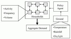
Figure 16. The structure of the water demand model
The neighbours in this model are defined as those in the n spaces orthogonally adjacent to a specified household as shown in Figure 17. The default value of this distance (n) used in the simulation was 4. The purpose of this neighbourhood shape was to produce a more complex set of neighbour relations than would be created using a simple distance-related neighbourhood (as in the Schelling model discussed above) while still retaining the importance of neighbour influence in the model.
Figure 17. The neighbourhood pattern for households in the water demand model
To give an idea of the social topology that results from this neighbourhood assumption we have shown the “most similar” neighbour influence pattern at a point in a typical run of the simulation in Figure 18 below. Due to the fact that every agent has a unique most influential neighbour, the topology of this social network consists of a few pairs of mutually most influential neighbours and a tree of influence spreading out from these. The extent of the influence that is transmitted over any particular path through the network will depend upon the extent that each node in that path is biased towards being influenced by neighbours rather than other sources (like the policy agent).
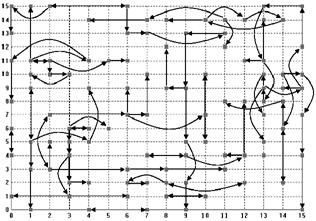
Figure 18. The most influential neighbour relation at a point in time during a typical run of the water demand model.
Households are also (but to a much lesser extent) influenced by all other households in their neighbourhood (as defined in Figure 17 above). Figure 19 illustrates all the effective neighbour relations between the households for the same time point in the same simulation run as shown in Figure 18. Note that the edges of this network are not wrapped around into a torus (as is often assumed in social simulation), so the households at the edges and corners have fewer neighbours that those in the middle. The reason for the chosen neighbourhood assumptions is that the resulting patterns (as in Figure 18 above and Figure 19 below) seem to us to be a reasonable mix of locality and complexity. We have no good empirical basis for this claim. It just seems intuitively right to us and we could not find any evidence about what the real structure is. (There have been some surveys done by the water companies that might provide evidence but they were not made available to the projects.)
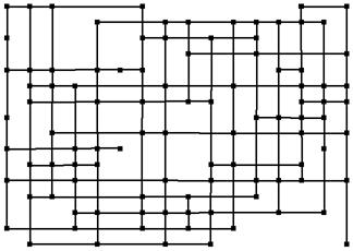
Figure 19. The totality of neighbour relations at the same point in time for the same simulation run as shown in Figure 18 using the neighbour definition given in Figure 17. (Each node connects to those 4 positions directly up, down, left and right on the grid.)
In each run the households are distributed and initialised randomly whilst the overall distribution of ownership and use of appliances by the households and their influence biases are approximately the same. In each run the same weather data is used so droughts will occur at the same time and hence the policy agent will issue the same advice. Also in each run the new innovations (like power showers) are introduced at the same date. Figure 20 shows the aggregate water demand for 10 runs of the model with the same settings (normalised so that 1973 is scaled to 100 for ease of comparison).
To illustrate the difference when the social network was disrupted, we ran the simulation again with the influence randomised in the same sense as it was in the P2P model described above. In this condition, the simulation had the same settings, social structures and so on except that whenever a household looked to other households, instead of perceiving the (public) patterns of water use for those households, the patterns of randomly selected households were substituted. Thus the neighbour-to-neighbour influence was always randomly re-routed in the second case. This does not affect the number of neighbours for each household, their cognition or the external factors. These all remain the same. All it does is randomise the structure of the network. In this way, we can observe what might be called a “pure” network effect. Figure 21 shows 12 runs of the randomised influence version of the model. This can be compared to Figure 20 where influence transmission occurs through networks.
Figure 20. The aggregate water demand for 10 runs of the model (55% neighbour biased, historical scenario, historical innovation dates, dashed lines indicate major droughts, solid lines indicate introduction of new kinds of appliances).
Figure 21. The aggregate water demand for 12 runs of the (otherwise identical) model where the neighbour influence relationship is “broken” by repeated randomisation.
The qualitative difference between the two runs is reasonably clear. In the first set of runs (Figure 20) there is an almost uniform reaction to droughts (and the advice of the policy maker) with nearly all runs showing a reduction in water demand during these periods. By contrast in the second set of runs (Figure 21) the reaction to such periods is not a general reduction in demand but rather a period of increased demand volatility. Secondly, the first set of runs shows much greater stability than the second set that exhibits short-term “oscillations” in demand even when matters are not complicated by a drought or the introduction of new water using technology.
What seems to be happening is that in the first model, smaller (and denser) neighbourhoods mutually influence each other towards a certain shared pattern, damping down any avalanches of influence that might otherwise take place. In the disrupted model, households “flip” between different patterns as the incoming influences vary resulting in a lot of noise. This influence noise acts to drown out the relatively “faint” suggestions of the policy agent. We would hypothesise that a “mean field” social influence model (in which each household perceives the average of water use patterns from neighbours) would be even smoother and more consistent in behaviour than the first model presented here. Thus the social influence in the model can be seen as somewhere “between” that of a randomised model and a mean field models sometimes used to approximate the dynamics in such cases. This is a situation that allows localised mutually reinforcing patterns of behaviour to compete with and influence other such localised patterns.
Elsewhere, Barthelemy (2003) shows that the output of this model is qualitatively and significantly affected by changes to the topology of the social network (including changes in the density of agents), by whether the space has edges (or is toroidally wrapped) and by the size of the agent neighbourhoods.
In any case it is clear that (as in the second case study) the structure of the social network does have a significant effect upon the resulting behaviour of the simulation beyond that indicated simply by the number of links each household has. If the system is randomised so the number of links stays the same but their arrangement displays no fixed pattern, the system outcome is very different. In this model, it appears to be the “lock in” of influence neighbourhoods rather than the structure of feedback loops that makes the distinctive character of the network significant. However, it is clear that in each case the underlying social generative process for the network is what leads to this effect. The characterisation of social networks by relatively simple egocentric measures may thus involve downplaying (or simply not thinking about) the fact that a dynamic social process underpins all social networks and this process, operating across a whole network, may display the distinctive character of a complex system.
Discussion
We have now presented three different simulation case studies and their characterisation by measured network properties. The case studies differ in how “theoretically” they represent a social system, what social system they represent, whether the networks involved are static or dynamic and how much “sociality” (communication, influence or reciprocation) each agent displays in its interactions. In each case, it appears that simple network measures must be treated with caution as characterisations of these systems. What should we conclude from this? It would be very easy to think of reasons to ignore the general argument of this paper. The models are not realistic, not typical or not very social, the measurements applied are naïve, the explanations of their failure are such as could have been offered by any moderately well trained SNA practitioner with good social intuition and without recourse to simulation. However, even if we grant all these points, we believe that this paper shows there is a case to answer and a novel tool to answer it with. The fact that we have not provided enough evidence to carry the argument in a single paper does not mean that we have provided no evidence at all. In future, we hope to provide further evidence, applying the approach to more models and examining more sophisticated characterisations but we hope too that this approach may appeal to other practitioners who will carry out work within the same programme. What then do we consider this programme to be?
Granovetter (1985) famously introduced the concept of embeddedness. Essentially embeddedness comes down to this: if an actor is socially embedded, then it is not satisfactorily represented using a model that ignores the particular structure of social relationships that the actor is involved in (Edmonds 1999). In other words, the behaviour of the actor can’t be reduced to interaction with a unitary environment (or set of identical others, which comes to the same thing) or to an individual acting on its own. It was concerns of precisely this kind that formed the background to the development of SNA – a concern to capture embeddedness and it effects and move away from the equally barren extremes of structuralism and individualism. However, the pragmatic difficulties involved in mapping complete networks (and an enthusiasm for technical issues) have resulted in the use of standard proxies for this structure in the shape of network measures – measures that can be more easily calculated and interpreted. Unfortunately, the broadly “statistical” approach to SNA seems to have drawn attention away from two crucial and related differences between networks and other objects of research. The first difference is that it is much harder to draw a clear distinction between measures and mechanisms. A set of cliques is simultaneously a characterisation of a network and the result of some underlying generative process that stands in need of explication. The second difference is that networks have the potential to be complex systems, making it very hard to anticipate how structured individual level interactions will “play out” to create macrostructure and too easy to apply inappropriate measures to the system in consequence.
In fact, there are (at least) two ways of using network measures. One may use them in a post hoc manner – that is, if one has a hypothesis or understanding about some social phenomena one then looks for appropriate means (including statistics on network measures) to test or illustrate this. Here, one has an idea of the mechanism and so is in a relatively good position to choose a measure (or other abstraction) that is suitable for highlighting or analysing the phenomenon. A possible danger is that one chooses an abstraction tending to confirm the hypothesis even if this is not representative of the phenomenon. For example, if one tries out a selection of centrality measures to see which one gives the strongest correlation one is seeking to demonstrate, one is assuming (without evidence) that the underlying regularity is as hypothesised. It may actually be that the weakest association proves a particular measure to be valuable because, in fact, there is no underlying causal mechanism to characterise.
The second way has a more a priori flavour. It is to use a network measure to gain an understanding of some phenomena at the outset. For example, by measuring the centrality of people with respect to some relationship in some social situation and then concluding something about the situation from this measure. The danger of this procedure is that in order to gain an understanding using such a measure, one has to assume a lot about its ability to represent something meaningful and known about the phenomenon one is trying to understand. However carefully one designs a measure, scaling it and adjusting it for various contingencies, there will always be networks and situations for which it gives a misleading impression (for any particular purpose).
Of course, most research in SNA advances through a pragmatic mixture of approaches that attempts to boot strap the understanding and clarity available. However, this does not absolve researchers from being more rigorous when communicating work to others – one has to try to untangle the complex web of steps that one used to achieve some understanding into one that is more amenable to criticism and careful checking.
A Way Forward: Using Simulation Models to Stage Abstraction
It is easy to criticise any abstraction on the grounds that it leaves out some aspect of the phenomena in question. We are not seeking to do this. We recognise the need for abstraction and simple description does not (in itself) progress understanding. If abstraction is not done explicitly it will occur anyway in an implicit manner. Humans are not able to perceive or read without automatically abstracting comprehensible “stories”.
However we are suggesting that abstraction can be staged and made less drastic through the use of descriptive social simulation models. We suggest that abstraction should be staged rather than jumping directly to network measures and their relations (which are the result of several progressive abstractions from the source phenomena). This staging occurs by starting with a descriptive social simulation of the phenomenon that can then be used as a basis for further abstraction to single (simulated) social networks and finally to a comparison of effective measures on those networks. This bottom-up process of building from phenomena towards higher abstraction (illustrated in Figure 22) can be seen as complementary to Carley’s call to make SNA more dynamic through the addition of agents (Carley 2003).
Figure 22. An illustration of the use of simulation to stage abstraction.
The following steps might constitute this staging process:
· Information about the dynamic and generative mechanisms could be collected by interviewing participants, stakeholders and experts as well as by direct observation (if this were possible).
· Other information (in the form of time series statistics) could be gathered regarding some of the outcomes of the model.
· A descriptive social simulation (that is one aiming to represent as much of the information as possible rather than trying to generalise more abstractly) would be built using the two collected sources of information as cross-validation (Moss and Edmonds 2005).
· Multiple runs of the simulation would be analysed to generate social networks and establish what can be meaningfully abstracted at this level.
· Measures that are designed to reflect the important aspects of the resulting social networks would be established, testing their interdependencies with outcomes and processes in the simulation.
· These measures could then be applied back to the original phenomena to observe their effectiveness and generality.
Like any methodological recipe, one should always be cautious of the applicability of “grand plans”, but it is hoped that this paper, by illustrating its points using a series of “working simulations” developed for other purposes has shown that the research process described above is not completely speculative. “Field” studies on the P2P model (and users of the software) to refine behavioural assumptions combined with quantitative monitoring of file transfer within a bounded domain (such as a university) would address the first two points. The (rather simple) P2P model already presented shows what kind of analysis can be carried out on a simulation. While the last two stages would have to wait for the development of a more empirically grounded model, we have at least hinted at how it might be carried out by showing the kind of negative findings that arise from inappropriate measures. We intend to provide a more detailed case study of this approach in a future paper.
References
Abbott, A. (2001) ‘Transcending General Linear Reality’, in Time Matters: On Theory and Method (Chicago, IL: The University of Chicago Press).
Barnett, G. A. (2001) ‘A Longitudinal Analysis of the International Telecommunication Network: 1978-1996’, American Behavioural Scientist, 44:1638-1655.
Barthelemy (2003) The impact of the model structure in social simulations. 1st European Social Simulation Conference, Gronigen, the Netherlands, 2003. (http://cfpm.org/cpmrep121.html)
Bolland, J. M. (1988) ‘Sorting Out Centrality: An Analysis of the Performance of Four Centrality Models in Real and Simulated Networks’, Social Networks, 10:233-253.
Bonacich, P. (1987) ‘Power and Centrality: A Family of Measures’, American Sociological Review, 52:1170-1182.
Borgatti, S. P., Carley, K. and Krackhardt, D. (forthcoming) ‘Robustness of Centrality Measures under Conditions of Imperfect Data’, Social Networks.
Carley, K. (2003) ‘Dynamic Network Theory’, in Breiger, R., Carley, K. and Pattison, P. (eds.) Dynamic Social Network Modelling and Analysis: Workshop Summary and Papers (Washington, DC: The National Academies Press).
Cohen, S. (2002) Folk Devils and Moral Panics: The Creation of the Mods and Rockers, third edition (London: Routledge).
Costenbader, E. and Valente, T. W. (2003) ‘The Stability of Centrality Measures When Networks are Sampled’, Social Networks, 25:283-307.
Downing, T. E., Butterfield, R. E., Edmonds, B., Knox, J. W., Moss, S., Piper, B. S. and Weatherhead, E. K. with the CCDeW project team (2003) Climate Change and the Demand for Water, Research Report, Stockholm Environment Institute (Oxford Office), Oxford, (http://www.sei.se/oxford/ccdew/).
Edmonds, B. (1999) ‘Capturing Social Embeddedness: A Constructivist Approach’, Adaptive Behaviour, 7:323-348.
Edmonds, B. and Moss, S. (2005) ‘From KISS to KIDS: An “Anti-Simplistic” Modelling Approach’, in Davidsson, P. et al. (eds.) Multi Agent Based Simulation IV, Lecture Notes in Artificial Intelligence Volume 3415 (130–144: Springer).
Edmonds, B. Bartheleny, O. and Moss, S. (2002) Domestic Water Demand and Social Influence – an agent-based modelling approach, CPM Report 02-103, MMU, 2002 (http://cfpm.org/cpmrep103.html).
Granovetter, M. (1985) ‘Economic Action and Social Structure: The Problem of Embeddedness’, American Journal of Sociology, 91:481-510.
Hedström, P. and Swedberg, R. (eds.) (1998) Social Mechanisms: An Analytical Approach to Social Theory (Cambridge: Cambridge University Press).
Ledeneva, A. V. (1998) Russia’s Economy of Favours: Blat, Networking and Informal Exchange, Russian, Soviet and Post-Soviet Studies 102 (Cambridge: Cambridge University Press).
Moss, S. and Edmonds, B. (2005) ‘Sociology and Simulation: Statistical and Qualitative Cross-Validation’, American Journal of Sociology, 110:1095-1131.
Schelling, T. (1969) ‘Models of Segregation’, American Economic Review, 59:488-493.
Williams, C. (2004) Cash-in-Hand Work: The Underground Sector and the Hidden Economy of Favours (Basingstoke: Palgrave).