Domestic Water Demand and Social Influence
– an agent-based modelling approach

Centre for Policy Modelling
Manchester Metropolitan University Business School

Introduction

This is a technical report to DEFRA and the EA as part of a deliverable by the CC:DEW project, coordinated by Tom Downing of the Stockholm Environment Institute.  The other technical reports that form the substantial part of this deliverable are concerned with forecasting the likely change in demand for water given certain changes in the climate.  This report is not to forecast but is to report on a more exploratory approach which has the potential to provide some of the possible deviations from the likely futures.

This reports starts with an introduction as to the nature of agent-based modelling and, in particular, what it is (and is not) suited to doing.  It outlines the structure of the model and briefly describes the results and finally states tentative conclusions.  Firm conclusions come in the form of what future work needs to be done.  There are four appendices with:  the graphs of the outcomes in terms of aggregate demand; detailed model specification; data sources and references.

The nature and use of agent-based modelling

Other parts of the CC:DEW project have been concerned with the expected change in the demand for water given certain levels of climate change.  These are based on a series of "surprise-free" predictions, extrapolating from current understanding of demand and its constraints.  They provide base lines on which to build future plans.  What they will not do is to capture new "non-linear" developments.  For example, that an increase in average temperature facilitates a fashion for automatically watered lawns.  However, climate change and its effect on demand are unpredictable, especially where it interacts with social processes (which are themselves unpredictable). 

When trying to plan for a situation that is known to be unpredictable it is sensible to be prepared for this fact.  One cannot predict the unpredictable, but what one can do is to try to consider some of the possibilities before hand.  Such preparation can enable the faster and more effective response should these occur.  For example, if one of the possibilities had rapid and extreme consequences it might be sensible to put into place monitoring processes to detect it, should it occur. 

Clearly, the usefulness of such an exercise depends upon the appropriate identification of what might happen.  Indicating essentially only one possibility by focusing only on what is reliably known means that one might not be prepared for qualitatively different outcomes.  Indicating too many possibilities by tracing out even wild and unlikely futures is also not likely to be helpful. 

The agent-based modelling work aims to indicate a few of the possibilities that are not merely deviations from the expected, but represent qualitatively different outcomes.  It aims to do this by using finer-grained models, with many different parts in the computer model (called "agents") separately representing different individuals and institutions.  Instead of the averaging of the outcomes being built into the model from the start (as in statistical models) any averaging to produce global summaries of outcomes occurs after the model has finished.  In other words, novel and qualitatively different outcomes are allowed to emerge from the interactions between the agents inside the model.  The hope is that these qualitatively different outcomes may pre-figure some of the real possibilities.

The aim of this kind of agent-based modelling is not to predict what outcomes will occur, and certainly not to capture all the real possibilities.  What it might be able to do is: (1) pre-figure some of the possibilities so that if something similar does occur we can be prepared for them (if only mentally) (2) to improve our understanding of the possible processes so that we are less often mislead and (3) to suggest important questions and further research to be investigate.

The technique has its disadvantages.  Producing credible future outcomes composed of believable interactions requires a lot of good information (both qualitative and quantitative) about the kind of interactions that actually occur.  Such models are inevitably complex and require a lot of checking in as many different ways as possible.  These models have a great many adjustable parameters and possible outcomes, so that a comprehensive set of runs covering all the possibilities is not usually feasible.  Finally there is the danger that the results (i.e. the indicated possibilities) might be over interpreted as if they were a prediction of might happen or a complete representation of what is happening. 

At this stage the agent-based models need a lot more development based on much richer information about the behaviour of the individuals and institutions concerned before the possibilities it indicates can be used in planning.  However, it does indicate some of the possibilities that might be sensible to check out with small field studies.  What it certainly does do is reveal the paucity of our knowledge of the decisions concerning water use that people make and how they make those decisions and that such differences in how decisions are made can result in very different outcomes given only very small changes in the environment.

The model set-up

This model focuses upon the behaviour of households, in particular how the household-to-household imitation of behavioural patterns may affect the aggregate demand for water.  Thus the heart of the model is a network of agents each of which represents a single household.  These are distributed randomly on a 2-D grid.  These ‘households’ can only interact with those with a certain distance of them.  The totality of households and their potential interactions can be considered to represent a community or cluster. 

The external environment for each household consists of: the temperature and precipitation; the exhortations of the water company; and, critically, the neighbouring households.  Each household has a number of different water-using devices such as: showers, washing machines, hoses etc.   The distribution and properties of these devices among households is done such that this matches a real distribution.  The output is the amount of water the households use.

The time is divided into months.  Each month, each household adjusts its water-using habits, in terms of the amount it uses each device, and whether it acquires new devices (such as power showers).  It does this adjustment based on the following: what devices it has; its existing habits; what its neighbours do (except for private devices such as toilets); and what the ‘policy agent’ (which is either the government or the water company) may be suggesting (in times of drought).  The weighting that each household uses for each of these is different and is set by the modeller.  In many of the runs it was set such that about 55% of the households were biased towards imitating a neighbour; 15% were predisposed to listen to the water company and the rest were largely immune to outside suggestion.  Obviously it is not known what proportions might be more realistic in terms of real communities, but anecdotal accounts suggest it varies greatly between communities. 

The “policy agent” represents the body responsible for issuing guidance to consumers as to water use in times of water shortage (currently this is the individual water companies in each area).  In the model there is a calculation of the level of ground water derived from the climatologically data, and the policy agent starts issuing suggestions during the second month where the ground is dry.  In subsequent dry month its suggestions are to use increasingly less water.

The model structure is illustrated below in Figure 1.

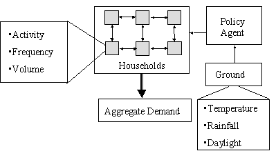
Figure 1: The General Structure of the Agent-based model

In this model there two new devices become available to the households: new washing machines (which use much less water than the older ones) and power showers (which use much more water than traditional UK showers).  These devices may be acquired by a household at any time after their becoming available, and in particular, when their existing device needs replacing.  The replacement rate of devices is estimated according using a Weibull distribution parameterised according to the type of device and an average life of 5 years.

What the Model Does Not Attempt to Cover

The model does not attempt to capture all the influences upon water consumption.  In particular it does not include any direct influence of the weather upon micro-component usage nor does it include any inherent biased towards increased usage due to background social norms such as increased cleanliness.  The behaviour of the policy agent is not sophisticated since it is the reaction of the households that is important here.

We had hoped to use some fine-grained data from Anglia Water which would have allowed us to specify any direct influence of micro-component data by the weather and any overall discernable trends in water consumption, however access to this data was not finalised at the time of writing.  It is hoped that this can be included in future developments.

Model Runs

Several sets of runs were done, in order to make three basic comparisons, namely to compare the runs with the UKCIP02 medium high emissions climate scenario for the mid-Thames region for 2050; the runs with different dates for the introduction of the new technologies; and the runs with different percentages of Neighbour biased households (i.e. those with a bias towards imitating their neighbours. 

The base case is with unmodified climate data for 1970-1997, with realistic dates for the introduction of power showers (4/90) and water saving washing machines (10/92), and with 55% of the population being biased towards imitating neighbours.

The first comparison is with a set of runs with the climate data modified so that it is consistent with the UKCIP02 medium-high emissions for the mid-Thames region for 2050 (see appendix 4 for details).

The second comparison is with a set of runs with different dates for the introduction of power showers (10/92) and water-saving washing machines (2/88).

The third and fourth sets of comparisons are with different proportions of neighbour-biased households, namely 30% and 80%.  Each of these comparisons was done with the unmodified and modified climate data.

Interpreting the results

When looking at the results, it should be recalled that the purpose of the model is to highlight qualitative differences that may arise.  The model is not designed to make accurate numerical predictions as to the likely outcome, but provide indications as to some of the possibilities.  In many ways exhibiting any graphs of the results is misleading, but they are included so that modellers and other experts can see the results.  They are displayed in appendix 2.

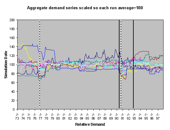
The simulations were done using data from 1970-1997, however many of the runs exhibited transient instability over the first year before they settled down into a definite pattern.  This behaviour is typical of this type of model, it occurs because of the lack of a long social history at the start of the simulation means that there are no social norms to constrain the model possibilities.  Given that there is great uncertainty about what kinds of socially grounded behaviour resulted in the past aggregate demand and that (in reality) there is a long social history to constrain the possibilities, we have discarded the first two years worth of resultant aggregate demand and scaled the resultant outcomes.  This is consistent with the fact that we are looking at qualitatively different outcomes rather than accurate levels.  We did the scaling in two ways: by scaling all the model outcomes so that the level at 1973 was 100 and by scaling each line so that its average level from 1973-1997 was 100. The former has the effect of lining up the outcomes at the start and the second has the effect of lining up the outcomes over the majority of its course.

Summary of the results

Although many of the outcome demand patterns were similar, there are a minority of runs which resulted in substantially different patterns.  In general, the higher the proportion of households that were biased towards imitating their neighbours, the more stable were the demand patterns, the more independent they were to suggestion and the greater affect the introduction of new innovations had.  In general, periods of drought (and hence exhortation by the policy agent to use less water) had a temporary effect, however in some runs this resulted in a permanent drop in demand.  This permanent drop in demand occurred more in the runs with the medium high emissions scenario.  In general the demands were less stable in the runs with using the medium high emission time series, i.e. they showed greater variety.

What the model indicates

The model does not tell us what people or communities will do, or even what they are likely to do.  Indeed in runs of the model we got a large variety of qualitatively different outcomes (in terms of the shape and size of aggregate domestic water demand), given a very simple range of simulated behaviours and exactly the same environmental conditions.  In the simulations certain behaviours can become established and then be robust against subsequent outside influence. This is because behaviours are imitated from simulated household to simulated household and so can become entrenched though mutual reinforcement.  Once this occurs, if the social reinforcement process is strong enough, the behavioural pattern can last for many years.

In the model runs periods of drought usually resulted in a slight and drop in demand, but this quickly reverted to previous levels.  In a very few runs the drought seemed to cause a significant and permanent drop in demand.  This suggests that it is possible that droughts might only have a long-term effect on household behaviour if the social conditions are right.

In general, differences in climate (such as might result from climate change in the medium term) did not usually cause a significant change in demand in this model, but in a few more runs there was a permanent drop in demand.  This does not suggest that climate won’t effect household behaviour but it does suggests that it is possible that the social effects within clusters of households may be a significant factor in determining the level of household demand, and so should not be ignored when considering climate effects.

In the runs the availability of new devices (such as new water-saving washing machines and power-showers) sometimes had a significant, but not completely predictable, impact on demand.  This suggests that it is possible that the availability of new products that are developed in response to climate change may have as profound an impact upon household water consumption as exhortation or direct climatologically effects on behaviour.

In the simulations the particulars of how the households were clustered and (socially) connected, and where the households looked to inform their behaviour substantially effected the outcomes in terms of demand.  Unfortunately, there is not much information concerning how people do behave in this regard, so as to inform the modelling of these aspects.  Thus the agent-based model points out the importance and potential of investigating such behaviour.  What would be required is a longitudinal study of household behaviour in small (100) clusters of households concerned with the purchase and use of water-consumptive appliances, in particular where consumers look to for suggestions in this regard.  This information might be extremely useful when trying to plan and direct public exhortation in situations of water shortage.   Whilst there has been considerable advance in the development of techniques to measure changes in the environment and water demand, there has been relatively little effort towards detecting social changes that may effect water demand.  The results from the agent-based model indicate that it is possible that social changes could be significant in their effect on domestic demand patterns.

Progressing the work further

Clearly there are several ways in which the model can be made more realistic.  To do this requires more and higher quality information about how households behave.  We had hoped to have access to Anglia Water’s SOPCON date, which gives a 15 minute reading of what devices were used for a sample of 100 “golden households”.  However it was not possible to gain access to this data in time for these results.  This sort of detailed longitudinal data is essential if good agent-based models of household behaviour are to be built.  Another aspect of which little is known is the topology of imitation networks in real neighbourhoods – a few detailed field studies of this would give us a handle on what real imitation processes might be occurring.

Acknowledgements

The original model was designed and implemented by Scott Moss with advice from Juliette Rouchier (now at GREQAM-CNRS).  It was then developed by Olivier Barthelemy, supervised by Scott Moss and Bruce Edmonds.  Bruce Edmonds made some minor modifications and did most of the runs reported here, he also wrote this report with help and contributions from Olivier Barthelemy.  The development of the model was supported, in part by the CC:DEW project which is funded by DEFRA and the EA.  CC:DEW is coordinated by Tom Downing, director of the Oxford branch of the Stockholm Environment Institute.  Both Tom Downing (SEI) and Cindy Warwick (ECI unit at Oxford) have given considerable assistance and advice.  We also acknowledge the support of the Manchester Metropolitan University Business School.  SDML was developed by Steve Wallis as part of an EPSRC/DTI ISIP project.  It was based upon a prototype written by Scott Moss.  It is written in Smalltalk/Visualworks and is freely distributable for academic and research use thanks to permission from Cincom who licences and distributes it.

Appendix 1 – Graphs of Aggregate Demand

Table 1 summarises the settings and the sets of runs done, each run takes between 6 and 18 hours to run with 40 households over the dates 1970-1997.

Table 1. Table of runs done

For each of these sets of runs we show two graphs of the resulting scaled aggregate demands.  The first of these is where the demands are scaled so that January 1973 is 100 units – this makes plain the deviations of the demands in the separate runs over the subsequent years.  In these graphs the broad line is the average of these.  The second graph is where each line is scaled so that the average of each resulting demand time series is 100 – this has the effect of ‘lining up’ the lines in the central region to facilitate their comparison.

For ease of reference the dates that innovations (i.e. power showers and water saving washing machines) are marked on the graphs as solid vertical lines and the most severe droughts shown as broken vertical lines.  In the historical climate scenarios these occur during the years of 1976 and 1990.  Under the medium high emissions scenario they occur during 1976, 1989, 1990, 1995 and 1996.

 

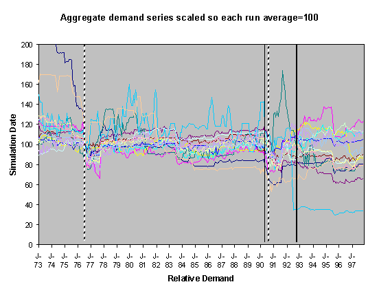
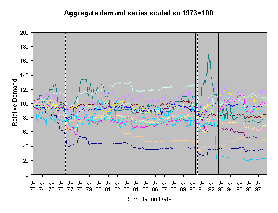
Figure 2.  30% Neighbour biased, historical scenario, historical innovation dates

 

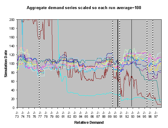
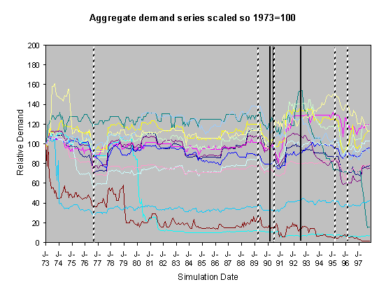
Figure 3.  30% Neighbour biased, medium-high scenario, historical innovation dates

 

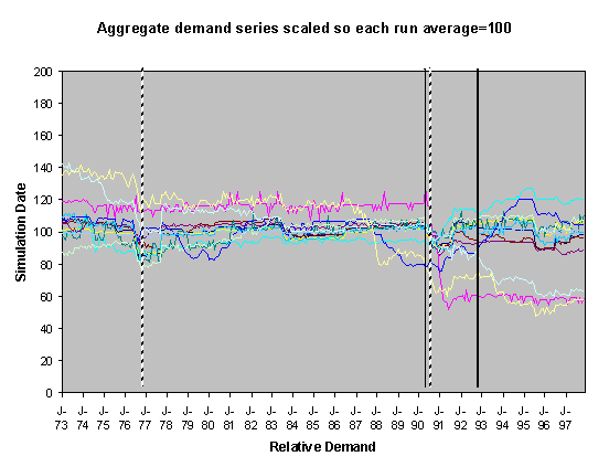
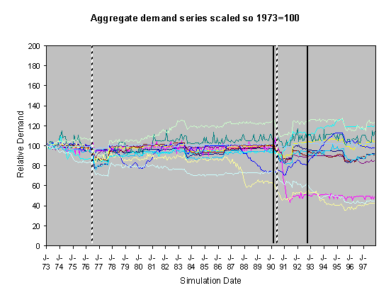
Figure 4.  55% Neighbour biased, historical scenario, historical innovation dates

 

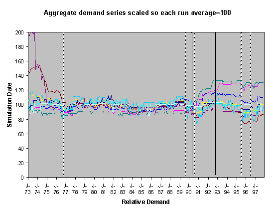
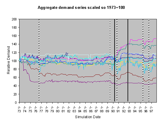
Figure 5.  55% Neighbour biased, medium-high scenario, historical innovation dates

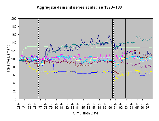Figure 6.  80% Neighbour biased, historical scenario, historical innovation dates

 

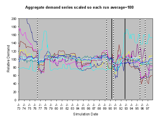
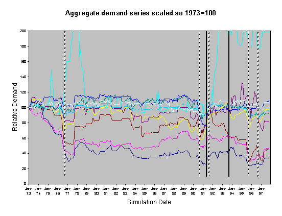
Figure 7.  80% Neighbour biased, medium high scenario,  historical innovation dates

 

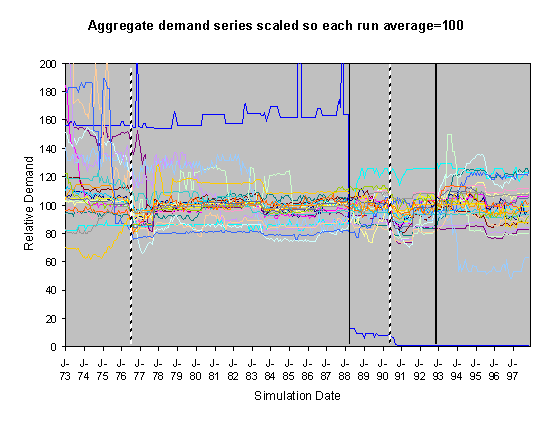
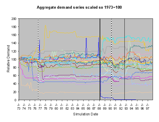
Figure 8.  55% Neighbour biased, historical scenario, changed innovation dates

Appendix 2 – Detailed Model Specification

Static Structure

The model container is iterated each month and each year for the designated time periods (in this case 1970-1997).  In this container the following sequence occurs: the ground module; the policy agent and the household cluster.  Preceding and following this sequence the model container does some administrative calculations such as reading the relevant climate data and calculating the resultant aggregate demand each month.  The container and sequence structure is shown in Figure 11.

 

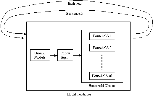
Figure 9. The agent and time structure of the model

The 40 households are executed in parallel, having access to others’ actions in previous but not current actions.  The households are randomly distributed about a 60×60 2D grid.  Each household can ‘observe’ the public actions of households within 4 squares of themselves horizontally and vertically.  An example such distribution is shown in 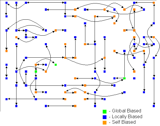Figure 10 (in this example a 16 by 16 grid with 100 housholds were used).

Figure 10. An example distribution of households (arrows show those households that are most influential to another)

Each household has a memory of possible actions and their endorsements, these include: the observable actions of its neighbours, the observable actions of the neighbour most like itself, the recommendations of the policy agent, its own past actions, its own recent past actions, and those for new applicances (with a low endorsement to introduce it).

Algorithms

This section outlines the model dynamics. The simulation time is composed of years and months.  For the purposes of this report we have restricted ourselves to recent history, 1973-1997.  Each month the following sequence is determined: Ground Water; Policy Agents; Household Decisions; and finally Aggregate Demand.  There are described below.

Ground Water

Each month, the ground water module calculates the moisture content of the ground using the modified Thornthwaite algorithm, using mean temperature, precipitation and sunshine time series.

The modified Thornthwaite algorithm is used to compute the soil moisture through potential evapotranspiration (PET) from temperature and hours of daylight per day (as in Food and Agriculture Organisation 1986).

The value of the unadjusted PET at temperatures above freezing is calculated as:

PET	Temperature (T) range
- 415,8547 + 32.2441T – 0.4325T2	26.5 ≤ T
16.5 (9 T / H) a	0 ≤ T < 26.5
0	T < 0

where H is heat defined as

and the exponent a is

6.75×10^-7 H³ - 7.71×10^-5 H² + 0.01792H + 0.49239

The day lengths are calculated from the day relative to the winter solstice and the latitude. The monthly PET values are adjusted to reflect the difference in water use between a grass surface and a mixed landscape of grass, trees and shrubs.  The monthly correction factors are:

 

Policy Agent

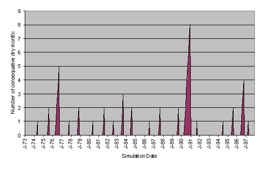
The Policy agent monitors the groundwater content calculated by the Ground Water module.  On a second consecutive month with less than 85% moisture content it starts to recommend the reduced use of water to the households.   The longer the dry period continues (i.e. as long as there is no month with 85% or more moisture content), the lower are the usages it recommends to the households.  The months of dryness characterised in this way is shown in Figure 11.

Figure 11.  Number of consecutive dry months in historical scenario

Household Decision Making

Each month each household updates its consumption patterns concerning the use of each micro-component.  It does this by considering its own actions, those of its neighbours, those of the neighbour that it considers is most similar to itself, the suggestions of the policy maker, and (in particular circumstances) possible new patterns with new appliances.  In the current model the consumption is not directly affected by the weather.

To decide among these the household uses an “endorsement” mechanism (Cohen, 1985), that is it remembers different suggestions as to the use of each micro-component along with its endorsement in the form of a label representing the source of the suggestion.  When it comes to making a decision it weighs up these suggestions using its own system of endorsement weights.  The set of base weights is randomly allocated to each household at the start of the simulation according to a distribution specified.  This distribution is specified by the expected percentage of households that are more biased towards imitating from neighbours, those that are more biased towards adopting suggestions by the policy agent, and those who tended to ignore either.  These biases do not determine behaviour rigidly, for example if it is not too biased towards listening to a policy agent if it has many neighbours which are suggesting a particular behaviour then this may “outweigh” the policy agent’s suggestion.

The approached used here, is to define a number base b and evaluate each endorsed object according to the formula

where e_i is a (usually integer) value associated with the i^th endorsement token. Negative values of endorsement tokens indicate naturally enough that they are undesirable. The higher the value associated with an endorsement token, the higher the class of tokens containing that particular token.  The value of b is the importance of an endorsement token relative to the value of a token in the class below. If the base is 2, then an endorsement of class three contributes 8 to the endorsement value of an object while an endorsement of class two contributes only 4.  For values of b larger than the number of tokens in any class used to endorse any object, the results from this evaluation scheme are the same as from Cohen’s evaluation scheme. For smaller values of b it is possible for a large number of lesser endorsements to outweigh a small number of endorsements of greater value.

Aggregation

The model adds together all the water use for all the households to produce the aggregate demand for that month.

Key Settings and Parameters

The most important settings are (setting options used in brackets):

• The size of the 2D grid (10);
• The number of households (40);
• The years over which the simulation is run (1970-1997);
• The range over which households can see each other (4 squares);
• The monthly average temperature and total precipitation time series (actual from Thames region; modified to be consistent with UKCIP02 medium high emissions scenario for 2050);
• The latitude (51°);
• The critical triggers for water use advice from the policy agent (85% moisture, 2^nd consecutive dry month);
• The available micro-components and their distribution among the households (from 3 Valleys data 1997/98);
• The dates for the introduction of new devices (4/90 power showers, 10/92 water saving washing machines or 10/92 power showers, 2/88 water saving washing machines);
• The proportion of households biased towards imitating from neighbours (30%, 55%, 80%);
• The proportion of households biased towards listing to suggestions from policy agent (15%);

Initialisation

The households are initially randomly distributed about the 2D grid.  They are initialised with water-consuming devices according to the given OVF distribution.  They are provided with a random set of weights (or biases) so that the population of households is divided up to match the parameters given.  They are given a minimal random set of behaviours that are minimally endorsed to start with.

Emergent Model Dynamics

An example of the how the endorsements affect the selection of a particular action from the first month of its adoption until it was replaced 6 months later, is shown in Table 2.  It shows how an action was reinforced by a combination of the endorsements: recent, neighbour sourced and self sourced (remembered, but not necessarily recent), until action-8472 eventually overtakes it by being neighbour sourced four times including being endorsed by the ‘most alike neighbour’.  How many neighbour sourced endorsements are necessary to ‘overcome’ endorsements such as ‘self sourced’ and ‘recent’ depends upon the weightings the agent is given during the model initialisation.

Table 2. An example of how endorsements may affect action choice

As a result of the learning and decision making by households, a self-reinforcing household-to-household imitation pattern can occur.  If the households are (on-the-whole) sufficiently biased towards imitating from neighbours then each household in a cluster may copy a substantial part of its behaviour from these neighbours who have copied the behaviour from their neighbours etc.  If the households are sufficiently clustered then patterns of behaviour may be copied back and forth, thus reinforcing itself.  Thus there is a sort of competition between different patterns of behaviour and the ‘locking-in’ of winning behaviour can result.

Appendix 3 – Data Sources

Climate time series

Monthly average temperature and total precipitation time series for Central England for 1970-1997 were used as inputs to the ground module, also a value for the latitude of 51° from which the hours of daylight are calculated.

Modifications to the climate time series to reflect the UKCIP02 medium-high emissions 2050 scenario

In order included a comparison of the outcomes under the UKCIP02 medium-high emissions 2050 scenario and current conditions the above time series were modified to reflect this UKCIP02 forecast for the upper Thames region.  This involved modifying the temperature and precipitation data as follows:

Table 3. Monthly modification to precipitation time series

Table 4. Monthly modification to temperature time series

Activity, Frequency, Use micro-component settings

The OVF data came from EA Strategies - Provincial Enterprise Scenario, Three Valley's Water - Resource Zone 2 for years 1997/98 and 2000/01.

Weibull parameterisations for micro-component replacement rates

The beta parameter, which determines the shape of the distribution, was taken from typical values given in (Bloch and Geitner, 1994).  The eta parameter is a scale parameter and was set so that the life expectancy of a device was 5 years.

Appendix 4 - References

 

Bloch, Heinz P. and Fred K. Geitner, (1994), Practical Machinery Management for Process Plants, Volume 2: Machinery Failure Analysis and Troubleshooting, 2nd Edition, Gulf Publishing Company, Houston, TX.

Brown, R. (1965) Social Psychology, New York: The Free Press.

Cohen, P. R. (1985) Heuristic Reasoning: an artificial intelligence approach. Boston: Pitman.

Environment, A. (2001). Water resources for the future : a strategy for England and Wales. p.84

Food and Agriculture Organization (1986). Yield Response to Water. Rome, FAO.

Herrington, P. and E. Great Britain Department of the (1996). Climate change and the demand for water. London, Hmso 1996.

Holman, I.P., Loveland,P.J., (eds.). (2002) REGIS: Regional Climate Change Impact Response Studies in East Anglia and North West England. Technical Report

Olivier Barthelemy, Scott Moss, Thomas Downing and Juliette Rouchier (2001) Policy Modelling with ABSS: The Case of Water Demand Management. CPM Report No. 02-92. http://cfpm.org/cpmrep92.html

Thornthwaite Charles, W. and R. Mather John (1955). The water balance. Centerton, N.J., Laboratory of Climatology.