Determining the Envelope
of Emergent Agent Behaviour via Architectural Transformation
*Centre for Policy Modelling, Manchester
Metropolitan University,
Aytoun Building, Aytoun
Street, Manchester, M1 3GH, UK.
Tel. +44 161 247 6478 Fax. +44 161 247 6802
{o.teran,b.edmonds,s.wallis}@mmu.ac.uk
†Department of Operation Research and Centre for
Simulation
and Modelling, Universidad de Los Andes.
Venezuela
Abstract. In this paper we propose a methodology to help analyse tendencies in
MAS to complement those of simple inspection, Monte Carlo and syntactic proof.
We suggest an architecture that allows an exhaustive model-based search of
possible system trajectories in significant fragments of a MAS using forward inference.
The idea is to identify tendencies, especially emergent tendencies, by
automating the search through possible parameterisations of the model and the
choices made by the agents. Subsequently, a proof of these tendencies could be
attempted over all possible conditions using syntactic proof procedures.
Additionally, we propose a computational procedure to help implement this. The
strategy consists of: unencapsulating the MAS so as to reveal the maximum
information about logical dependencies in the system. This information is
maximised by splitting the transition rules by time intervals and some
parameters. An example applying this procedure is exhibited which ‘compiles’
the rules into this form. In the example the exploration of possibilities is
speeded up by a factor of 14. This
makes possible the complete exploration of model behaviour over a range of
parameterisations and agent choices.
1 Introduction: Understanding MAS
MAS
can (and frequently do) exhibit very complex behaviour – in this fact lies their
promise but it also means that they can be difficult to understand and predict.
Broadly there are two means by which we can seek to understand MAS: through
design and through observation. Careful design procedures based on
well-understood formal models of agent behaviour help us to understand the
behaviour of individual agents and, in special cases, larger parts of MAS.
However understanding the behaviour of interacting groups of autonomous agents
by formal design methods has its limitations, and even the most carefully
designed MAS can exhibit emergent behaviour unforeseen by its designers. This
is hardly surprising as half the point of
autonomous agents is that they should be able to deal with circumstances
unforeseen by their designers.
Thus a second
important way in which we can control MAS (after careful design) is by
inspecting and analysing the behaviour of MAS in a post hoc manner, so that this can inform our future design and
control of them. In other words, just like any software development environment,
to effectively deploy MAS one needs both design and debugging tools. The most common methods of such post hoc
analysis are: firstly, by detailed
scenario analysis, where a single MAS trajectory at a time is examined and
analysed and secondly, using a Monte
Carlo approach where the MAS is repeatedly run and statistics collected about
general trends over a sample of trajectories.
The scenario analysis
provides the richest source of
information, typically providing far more detail than the programmer can
possibly cope with. It is also inherently contingent and it can be difficult to
separate out what can be taken as representative behaviour and what is
exceptional. After examining and interacting with several such runs of the
system it is up to programmers to abstract an understanding of the MAS’s
behaviour using their intuition; the scenario analysis only conclusively
demonstrates possibilities.
A Monte Carlo approach
can be used to separate out the exceptional from the representative in some
cases, but has a number of drawbacks including: the sort of behaviour one is
investigating may not be satisfactorily summarised using numerical devices (for
example in safety critical systems it may be insufficient to know that a
certain parameter probably stays
within an acceptable range, on would want to know it does); and the use
of statistics inevitably involves the use of certain assumptions, which may not
always be appropriate.
In this paper we
discuss the use of a constraint-based search of possible models which can be
deployed on significant subspaces of the total space of MAS possibilities. Like
the Monte Carlo approach this can be seen as falling half-way between syntactic
proof procedures and single scenario analyses. Unlike the Monte Carlo approach
it produces definite answers to questions relative to the chosen subspace of
possibilities – it can be seen as model-based proof w.r.t. subsets of the
possibilities. It does not magically solve the problems in understanding all
emergent MAS behaviour but is a useful addition to our menu of tools because it
embodies a different trade-off between semantic richness and computational
efficiency.
We will begin in
section 2, by outlining the main idea.
The implementational concerns of the technique, i.e. the proposed
architecture for doing the constraint-based model search in a “hunt” of
tendencies is described in section 3. Following this (section 4), we will give
an example of applying this architecture. Then in section 5, we will compare
this procedure with a couple of related approaches. In section 6 we briefly
position this approach with respect to single simulation inspection and general
theorem proving. Finally, some conclusions are made.
2 Exploring the
envelope of emergent MAS behaviour
We want to be able to establish a more general type of knowledge of emergent behaviour than can be gained from the inspection of individual runs of a system. In particular we want to know whether a particular emergent behaviour is a necessary consequence of the system or merely a contingent one. Thus we propose to translate the system from an agent formulation into a form whereby the envelope of system possibilities can be determined, under a wider range of conditions. The target we have chosen is a constraint-based architecture: the MAS, modulo a range of parameterisations and nondeterministic agent choices, are translated into a set of positive constraints and the inference engine then searches for a model (i.e. a representation of a possible simulation in the original MAS with a particular parameterisation and set of choices) that satisfies these. This establishes the consistency of the positive constraints[1]. Postulated formulations of general emergent behaviour can be tested as to their necessity over the range of parameterisations and nondeterministic choices by negating them and adding them as a further constraint followed by getting the system to check that there is now no possible model.
The idea is to do this in a way which makes it possible to translate the MAS into the constraint-based one in an automatic or near automatic way without changing the meaning of the rules that make it up. In this way a user can program the system using the agent-based paradigm with all its advantages, inspect single runs of the system to gain an intuitive understanding of the system and then check the generality of this understanding for fragments of the system via this translation into a constraint-based architecture.
3
Implementing a
suitable constraint-based architecture
The main goal of the programming strategy to be described is to increase the efficiency in terms of simulation time, thus making the constraint search possible. The improvements will be achieved by making the rules and states more context-specific. This enables the inference engine to exploit more information about the logical dependencies between rules and thus increase the efficiency. Thus this can be seen as a sort of ‘practical compilation’ process which undoes the agent encapsulation on an implemented MAS system in order to allow the more efficient exploration of its behaviour. In particular we split the transition rules into one per simulation period, and also by the initial parameters. This necessitates a dynamic way of building rules. This is done via a controller which generates the rules at the beginning of the simulation.
3.1 Time Discrete Simulation Approach
In
synchronous simulations, time is taken as a discrete variable, given here as a
set of positive numbers. In our case, we will call any of these numbers where
the state variables are recalculated, a simulation time instant (STI) and the
amplitude of the interval between two consecutive numbers, a simulation time
step (STS). The transition function determines the state variables for STIs
using the known values of the state variables in previous STIs. It is assumed
that the state variables remain constant between two consecutive time instants.
In this architecture the structure of the simulated system is more than the one usually described in simulation formalisations (see for example Zeigler, 1976), e.g., it allows certain forms of structural change. A meta-agent as a controller in a MAS could guide not only quantitative changes, but also qualitative ones admitting its introduction into an evolutionary environment in a modular and transparent manner.
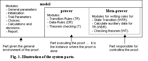
3.2 Overview of the Architecture
We
implemented the proposed architecture in three parts, let us call them model, prover and meta-prover
(we happen to have implemented these as agents but that is not important). The
following illustrates this:
3.3
Program dynamics
The
system fires the rules in the following order:
1.
model: initialising the environment for the proof (setting parameters, etc..)
2.
meta-prover: creating and placing the transition rules in prover.
3.
prover: carrying on the simulation using the transition rules and backtracking
while a contradiction is found.
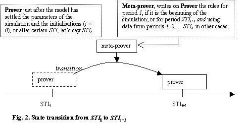 The program backtracks from a path once the
conditions for the negated theorem are verified, then a new path with different
choices is picked up. The next figure describes a transition step.
The program backtracks from a path once the
conditions for the negated theorem are verified, then a new path with different
choices is picked up. The next figure describes a transition step.
3.4 Description of
System Modules
General Parameters (GP). This will be placed in the model (see figure 1). Its task will be to set the general
parameters of the simulation.
Initialising (I). This creates the entities (e.g. agents) given
the static structure of the simulation and initialises the state variables for
the first STI. It will be in model,
as it is responsible for initialising parameters to be instantiated by meta-prover when writing the transition
rules.
Trial Parameters (TP). To be placed in the model. Its task is to set up parameters to be fixed during one
simulation trial. In general these are parameters for which the agents do not
have to take decisions every STI (as for GP). They would be fixed before
creating the transition rules.
Choices (CH). It will place alternatives for the choices the agents have every STI
and the conditions under which each choice could be made. Choices will be
mainly responsible for the splitting of the simulation and the rise of
simulation branches.
Data Rules (DR), and Calculations and Decision
rules (C&D). The first module would contain the set of
rules responsible for doing calculations required by the transition rules and
which is worthy to keep in the database (they could evolve like the TR). The
second one is a sort of function generating a numerical or a truth value as a
result of consulting the database and usually consists of backward chaining
rules.
Theorem (Constraints)(T). These are the conditions for checking the
theorem. The theorem will be examined by a rule written by meta-prover in prover.
Reports (R). The purpose of this module seems to be simple: to give the user outputs
about what is going on in the dynamic of the simulation. This module will
allows the user to know facts about the branch being tested as well as about
branches already tested.
Transition Rules (TR). This is the set of rules will be context
dependent and will include explicitly syntactical manipulation to make more
straightforward the linking among them.
3.5 Split of the rules:
a source of efficiency
A
graphical illustration of the split procedure would be:
In forward
chaining simulation the antecedent retrieves instance data from the past in
order to generate data for the present (and maybe the future):
past facts à present and future facts
Traditionally, the set
of transition rules are implemented to be general for the whole simulation. A
unique set of transition rules is used at any STI.
As the simulation
evolves, the size of the database increases and the antecedents have to
discriminate among a growing amount of data. At STIi, there would be data from (i-1) alternative days matching the antecedent. As the simulation evolves it becomes slower because of the
discrimination the program has to carry out among this (linearly) growing
amount of data.
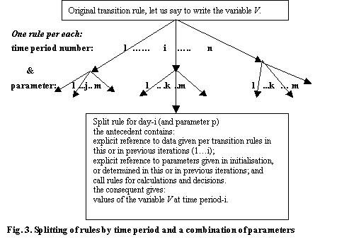 Using the proposed technique, we would write a
transition rule for each simulation time. The specific data in the antecedent
as well as in the consequent could be instanced. Where possible, a rule for
each datum, the original rule will generate, would be written. This will be
better illustrated in the example of the next section.
Using the proposed technique, we would write a
transition rule for each simulation time. The specific data in the antecedent
as well as in the consequent could be instanced. Where possible, a rule for
each datum, the original rule will generate, would be written. This will be
better illustrated in the example of the next section.
This technique
represents a step forward in improving the efficiency of declarative programs,
one could, in addition, make use of partitions and time levels. Partitions
permit the system to order the rules to fire in an efficient way according to
their dependencies. Time levels let us discriminate among data lasting
differently. The splitting of rules lets
us discriminate among the transition rules for different simulation times given
a more specific instancing of data at any STI.
3.6 Measuring the
efficiency of the technique
Comparing
the two programs, the original and the one where the technique was implemented,
in terms of the amount of data the program has to search into in order to check
if a rule fires, we could have a rough idea about the increase in speed given
by the technique.
While in the efficient
program, each rule instances the specific data necessary to generate each datum
at each STI, in the original one it has to discriminate among STIs and other
not explicitly specified entities. For
example, if there were three instances of 'producer', and the antecedent of a
rule refers to 'producer', the rule has to discriminate among the three
instances. This does not happen when using the technique. So, if there are N
instances of any entities in certain rule, the technique speeds up the
simulation in a factor of N when firing such a rule. Similarly, the technique
speeds up the simulation by discriminating among STIs.
The technique allows a
speed by a factor of NM/2. SDML
already has facilities for discriminating among STIs, but their use is not
convenient for the sort of simulation we are doing (exploring scenarios and/or
proving) because of the difficulties for accessing data from any time step at
any time. If we had used this facility in the original simulation model, it
would have been speeded up by MN(M-1)/2.
It is clear that the
greater the number of entities in the simulation or the number of STIs, the
larger the benefits the technique gives. We must notice that the speeding up of
the simulation is only one aspect of the efficiency given by the technique.
3.7 Translating a traditional MAS architecture
into a model-exploration MAS architecture.
Before
splitting the rules the original MAS is reduced in a sort of unencapsulation of the hierarchy of
agents into the architecture shown in figure 1. Additional variables must be
added into predicates and functions in order to keep explicit the reference to
the "owner" agent of any instance of a variable. This will facilitate
the check for tendencies, the testing of the theorem and any other data
manipulation. It is as if the agent where replaced by its rulebase, see figure
4.
In the original
architecture, each agent has its own rulebase (RB) and database (DB). The
agent's structure is given by its set <RB, DB> as well as by the
structure of any subagents.
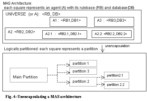
Using the technique, the initialisation of the static structure is accomplished
by the module "Initialising", as explained above. The transition
rules (dynamic structure) will be situated in the module "Transition
Rules". There is still a
hierarchy, both in the structure of the model and in the dynamics of the
simulation – it is given by the precedence in the rulebase partition (figure
4).
Now we turn to show a
way of implementing the technique automatically. After adding variables to
associate data with agents, the task is to write it modularly, as illustrated
in figure 4. One of the key issues is to determine dependencies among rules and
then choose appropriate data structures to allow the meta-prover to build the
TR. A procedure to do it would be:
1.
Identify
parameters and entities for splitting (agents and/or objects) as well as the
dependencies among rules. Look for a "general" description of the
dependencies. E.g. a Producer's price at STIi
depends on Producers' sales and prices at STIi-1.
2.
Create a list of
references or links to each datum used in dependencies. Taking the previous
example, a list containing the names of the clauses for prices and sales is
created ([Price1, Price2
…, Pricen], [Sale1,
Sale2, …, Salen] (Pricei,
refers to price at STIi).
This list could be also specified by producer, if necessary.
3.
Initialise
parameters (GP and TP) and data at STI1.
It would be a task of module I (see above). It creates data used by module WTR
at meta-prover and which are input
for TR at STI2.
4.
Provide the
values for the choices the agents have.
5.
Using these data
structure and our knowledge about dependencies, we must be able to write the
WTR, WDT, and WT at meta-prover. If
TR at STIi depend on data
at STIi-1 then the list
named in 2. would allow to make such a reference automatically accessing the
appropriate elements in the list.
6.
Modules like R,
C&D are auxiliary and do not need special attention.
Constraints in the search are applied in different ways, for example when theorem
is adapting (maybe relaxing conditions for a tendency) and as WTR and WDR take
into account the past and present dynamic of the system (for instance, when
restricting choices for the agents or objects, constraining the space of
simulation paths).
3.8 The platform used
We implemented the systems described entirely within the SDML programming language[2]. Although this was primarily designed for single simulation studies, its assumption-based backtracking mechanism which automatically detects syntactic logical dependencies also allows its use as a fairly efficient constraint-based inference system. SDML also allows the use of “meta-agents”, which can read and write the rules of other agents. Thus the use of SDML made the procedures described much easier to experiment with and made it almost trivial to preserve the meaning and effect of rules between architectures. The use of a tailor-made constraint-satisfaction engine could increase the effectiveness and range of the techniques described once a suitable translation were done, but this would make the translation more difficult to perform and verify.
A
simple system of producers and consumers, which was previously built in SDML
and in the Theorem Prover OTTER, was rebuilt using the proposed modelling
strategy. In the new model the exploration of possibilities is speeded up by a
factor of 14.
Some of the split
transition rules were the ones for creating (per each STI) producers’ prices
and sales, consumers’ demand and orders, warehouses’ level and factories’
production. Among the rules for auxiliary data split were the ones for
calculating: total-order and total-sales (a sum of the orders for all
producers), total-order and total-sales per producer, and total-order and
total-sales per consumer.
4.1 Example of a split
rule: Rule for prices
This
rule calculates a new price for each producer at each STI (which we called day), according to its own price and
sales, and the price and sales of a chosen producer, at the immediately
previous STI.
The original rule in
SDML was like this:
for all (producer)
for all (consumer)
for all (day)
(
price(producer,myPrice,day)
and
totalSales(totalSales,day)
and
sales(producer,mySales,day) and
choiceAnotherProducer(anotherProducer) and
price(anotherProducer,otherPrice, day) and
calculateNewPrice(mySales,totalSales, otherPrice, myPrice,newPrice)
implies
price(producer, newPrice, day + 1)
)
The new rule (in the
efficient program) will be “broken” making explicit the values of prices and
sales per each day.
In the following, we
show the rule per day-i and producer-j:
for all (consumer)
(
price(producer-j, myPrice, day-i) and
totalSales(totalSales, day-i) and
sales(producer, mySales, day-i) and
choiceAnotherProducer(anotherProducer) and
price(anotherProducer, otherPrice, day-i) and
calculateNewPrice(mySales,totalSales,otherPrice,myPrice,newPrice)
implies
price(producer-j, newPrice, (day-i) + 1)
)
If the name of price
is used to make explicit the day, the rule will have the following form. It is
important to observe that only one
instance of newPrice in the consequent is associated with only one transition
rule and vice verse:
for all (consumer)
(
price-i(producer-j, myPrice) and
totalSales-i(totalSales) and
sales-i(producer-j, mySales) and
choiceAnotherProducer(anotherProducer) and
price-i(anotherProducer, otherPrice) and
calculateNewPrice(mySales,totalSales, otherPrice, myPrice,newPrice)
implies
price-(i+1)(producer-j, newPrice)
)
4.2 What the technique
enables
In
this example, we used the technique to prove that the size of the interval of
prices (that is: biggest price - smaller
price, each day) decreased over time during the first six time intervals
over a range of 8 model parameterisations. An exponential decrease of this
interval was observed in all the simulation paths. All the alternatives were
tested for each day - a total of 32768 simulation trajectories. It was not
possible to simulate beyond this number of days because of limitations imposed
by computer memory. There was no restriction because of the simulation time, as
the technique makes the simulation program quite fast – it had finished this
search in 24 hours.
This technique is useful not only because of the
speeding up of the simulation but also for its appropriateness when capturing
and proving emergence. On one hand, it let us write the transition rules and
the rule for testing the theorem at the beginning of the simulation in
accordance to the tendency we want to prove. And, on the other hand, if the
meta-prover is able to write the rules while the simulation is going on, it
could adapt the original theorem we wanted to prove according to the results of
the simulation. For example, if it is not possible to prove the original
theorem then it could relax constraints and attempt to show that a more general
theorem holds. Moreover, the technique could be implemented so that we have
only to give the program hints related to the sort of proof we are interested
in, then the meta-prover could adapt a set of hypotheses over time according to
the simulation results. At best, such a procedure would find a hypothesis it
could demonstrate and, at worst, such output could then be useful to guide
subsequent experimentation.
In
OTTER (and similar Theorem Provers) the set of simulation rules and facts
(atoms) is divided into two sets (this strategy is called support strategy) (McCune 1995):
One set with “support”
and the other without it. The first one is place in a list called “SOS” and,
the second one, in the list “USABLE”. Data in USABLE is “ungrounded” in the
sense that the rules would not fire unless at least one of the antecedents is
taken from the SOS list. Data inferred using the rules in USABLE are placed in
SOS when they are not redundant with the information previously contained in
this list, and then used for generating new inferences. The criteria for
efficiency are basically subsumption and weighting of clauses.
Rules are usually
fired in forward chaining but backward chaining rules and numerical
manipulations are allowed in the constructs called “demodulators” (Wos, 1988).
In simulation
strategies like event-driven simulation or partition of the space of rules, in
declarative simulation, are used. The criteria for firing rules is well
understood, and procedures like weighting and subsumption usually are not
necessary. Additionally, redundant data could be avoided in MAS with a careful
programming.
The advantages given
for the weighting procedure in OTTER are yielded in MAS systems like SDML by
procedures such as partitioning,
where chaining of the rules allows firing the rules in an efficient order
according to their dependencies.
Among other approaches
for the practical proof of MAS properties, the more pertinent might be the case
conducted by people working in DESIRE (Engelfriet et. al., 1998). They propose
the hierarchical verification of MAS properties, and succeeded in doing this
for a system.
However, their aim is
limited to verification of the computational program – it is proved that the
program behaves in the intended way. It does not include the more difficult
task, which we try to address, of establishing general facts about the dynamics
of a system when run or comparing them
to the behaviour observed in other systems (Axtell et al., 1996).
6
A sequence of architectures for modelling behaviour and proving theorems in MAS
The
architecture we describe could be used after single simulations have been run
to suggest useful properties to test for. Subsequently
one could employ a syntactically oriented architecture for proving those
tendencies outright. Thus the proposed
technique can be seen as falling in between inspecting single runs and
syntactic theorem proving. This is illustrated in figure 5.
The step to theorem
proving from model-based exploration would involve a further translation step.
The conditions established by experimenting with model-based 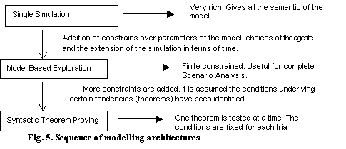
exploration would need to be added to the
MAS specification and all this translated into axioms for the theorem prover to
work upon. The main aspects of the three architectures are summarised in Table 1, which is a comparison of these different approaches.
|
Architecture: Aspect: |
SCENARIO |
MODEL-EXPLORATION |
SYNTACTIC |
|
Typical paradigm |
Imperative. |
Constraint |
Declarative |
|
Typical deduction system |
(Forward Chaining) |
Forward Chaining using efficient
backtracking |
Backward chaining or
resolution-based |
|
Nature of the manipulations |
Possible Semantic |
Range of Semantics |
Syntactic |
|
Limitations |
Not constrained. - Very rich. Too much
information could mislead |
- Finite constrained. Still
quite rich. - Suitable for Scenario
Analysis. |
-Constrained. - Valuable for proving specific
tendencies. |
|
Search style. |
Attempts to explore all
simulation paths. |
Limits the search by
constraining the range of parameters and agent choices |
Can be efficient in suitably constrained
cases, typically impractical |
Table 1. A Comparison of Architectures
7 Conclusion
The
proposed methodology is as follows: firstly,
identify candidate emergent tendencies by inspection of single runs; secondly, explore and check these using
the techniques of constraint-based model-search in significant fragments of the
MAS; and finally, attempt to prove
theorems of these tendencies using syntactic proof procedures. This methodology is oriented towards
identifying interesting tendencies and emergence in MAS an area little explored
but of considerable importance.
In addition,
we have proposed a framework for improving the efficiency of MAS to enable the
second of these. It has been implemented in an ideal example, resulting in a
significant increase in the speed of the program. However, the notions are
valid independently of the example and could be implemented in many different
systems. In summary, the strategy consists of: unencapsulating the MAS system
to allow the maximum amount of dependency information to be exploited;
partitioning of the space of rules and splitting of transition rules by STI and
some parameters, using the appropriate modularity of the simulation program,
and specially initialising parameters and choices.
The technique perhaps
presages a time when programmers routinely translate their systems between
different architectures for different purposes, just as a procedural programmer
may work with a semi-interpreted program for debugging and a compiled and optimised
form for distribution. In the case of
agent technology we have identified three architectures which offer different
trade-offs and facilities, being able to automatically or semi-automatically
translate between these would bring substantial benefits.
Acknowledgements. SDML has been developed in
VisualWorks 2.5.2, the Smalltalk-80 environment produced by ObjectShare. Free
distribution of SDML for use in academic research is made possible by the
sponsorship of ObjectShare (UK) Ltd. The research reported here was funded by
CONICIT (the Venezuelan Governmental Organisation for promoting Science), by
the University of Los Andes, and by the Faculty of Management and Business,
Manchester Metropolitan University.
References
Axtell, R., R. Axelrod, J. M. Epstein, and M.
D. Cohen (1996), “Aligning
Simulation Models: A Case of Study and Results”, Computational Mathematical
Organization Theory, 1(2), pp. 123-141.
Engelfriet, J., C. Jonker and J. Treur (1998) “Compositional Verification of Multi-Agent
Systems in Temporal Multi-Epistemic Logic”, Artificial Intelligence Group,
Vrije Universiteit Amsterdam, The Netherlands.
McCune, W. (1995), OTTER
3.0 Reference Manual Guide, Argonne National Laboratory, Argonne, Illinois.
Moss, S., H. Gaylard, S. Wallis, B. Edmonds
(1998), “SDML: A Multi-Agent
Language for Organizational Modelling”, Computational Mathematical Organization
Theory, 4(1), 43-69.
Wos, L. (1988), Automated
Reasoning: 33 Basic Research Problems, Prentice Hall, New Jersey, USA.
Zeigler, B. (1976), Theory of
Modelling and Simulation, Robert E. Krieger Publishing Company, Malabar, Fl, USA.