The impact of the model
structure in social simulations
O. Barthélémy
Centre for Policy Modelling, Manchester
Metropolitan University,
O.Barthelemy@mmu.ac.uk
The use of scenarios for planning
is quite common, be it for industries, nations, shop chains, or technologies.
They represent a specific approach where while dealing with uncertainties, one
can either consider the whole (frequently continuous) range of alternatives, or
specify particular cases that would capture key properties of this range.
From their appearance in the
literature in the 40s, scenarios have been more and more frequent. It was
generally extrapolated through past data and relationships, till the 80s, when
the studies in innovation and diffusion showed that the future is depending on changes
in social and economic systems which paths are multiple, and indeed not fixed,
but evolving themselves. The goal of scenarios then became the analysis of some
trends within a “possibility space”, and eventually the reduction of that space
finding potential discontinuities, in order to improve the decision making
process.
It is the case for climate change
and social behaviour throughout time. Scenarios are used because the future is
uncertain, and the ability to adapt to these future changes might have effects
upon the longer term (e.g. technological changes).
A multi agent system can be used
to represent formally these scenarios and its structure and components can then
be analysed in order to evaluate their impact upon the outcome.
The interest in scenarios
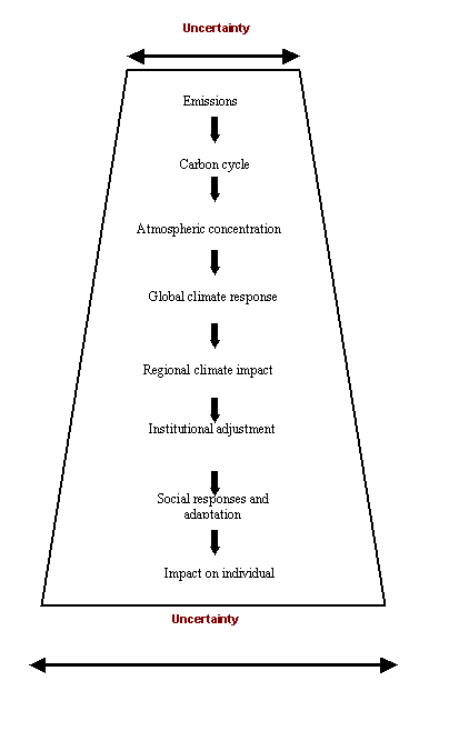
This diagram from the CC:DEW report
shows the increasing uncertainty as the different components are integrated
into a model.
Fig 1: The presence of uncertainty at
multiple levels
Multiple scenario frameworks are
built on the Environmental Futures scenarios, from the UK Foresight
programme. This programme tries to look beyond normal commercial horizons to
identify potential opportunities from new science and technologies. It intends
to deliver thorough and up to date information and analysis of recent
developments in relevant science and technology, vision of the future
reflecting the potential impact of science and technology and of forecast
social and economic trends, recommendations for actions, and networks of people
who recognise the importance of the issues addressed by the project.
The Foresight Future scenarios
have been created for the UK Foresights programme, and the project was funded
by the Department of Trade and Industry, as well as the Department of
Environment, Transport and the Regions. The research was led by the Science and
Technology Research Policy for the UK Foresight Programme (SPRU) from the
University of Sussex. These scenario represent a tool for foresight, enabling
institutions, businesses, and more generally users, to apprehend possible
futures, in order to improve their decision making.
Generated via an iterative
participatory process, the scenario framework also draw on pre-existing work,
such as the scenarios developed by the Intergovernmental Panel on Climate
Change (IPCC 2000) that is trying to estimate
future greenhouse gas emissions.
The UKCIP scenarios use computer
estimations of climate change, and are attempting to assess their impact upon
the UK’s socio-economic structure. They differ from the Foresight scenarios by
being specifically designed for the timescale of the associated climate
scenario provided, and by providing details likely to be of use for regional
and sectoral studies. For example, they give greater emphasis to the possible
changes to regions and to certain types of geographical domain. Classified
according to governance system and social values, their denomination is
equivalent to the Foresight scenarios, apart from the Provincial Enterprise,
renamed National Enterprise. Every scenario describes a plausible future, and
the shape of water demand, agricultural trends, future transport, and economic
development.
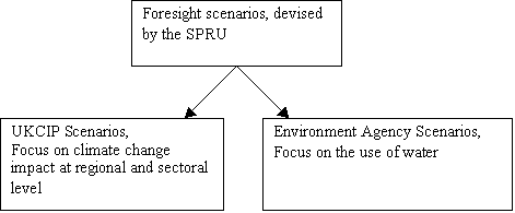 The scenarios presented by the Environment agency are based upon the
UKCIP scenarios, themselves based on the Foresight scenarios. The Foresight
scenarios were devised taking into account various sectors of the economy. The
UKCIP focused on the climate change impact, and the EA focused further on water
resources.
Fig 2: The different focuses of
studies originating from the future scenarios
Four distinct Foresight scenarios
were retained as typical cases. They are classified according to a couple of
main indicators, or drivers of change: the social values of the individuals,
and the governance structure in place.
Social values go from individualistic to
more community oriented, while the system of governance, dealing with the
structures of the government and the decision making process go from autonomy
(power remaining to national level) to interdependence (power moves to
institutions, e.g. from the EU to regional government).
|
Governance \ Values |
Individual |
Community |
|
Interdependence / Globalisation |
World Markets (B) |
Global Sustainability (C) |
|
Autonomy / Regionalisation |
Provincial Enterprise (A) |
Local Stewardship (D) |
The scenarios have specific
general characteristics, presenting the general trends, and more details upon
economic and sectoral trends, employment and social trends, regional
development, health, welfare and education, and the environment.
The statistical issue
As clearly expressed in
Herrington (1996), the statistical results obtained for a given period, and the
best goodness of fit for several representations were varying when applied to
the following time period, largely reducing the interest of such results in a
forecasting perspective. One of the reasons for such lack of success could be
the fact that the tools might not be appropriate for the subject of study.
The use of parametric statistics,
although very common, is subject to several conditions.
It includes the fact that both
variables should have homogeneous levels of variance. Parametric statistics use
the knowledge upon the distribution the sample is extracted from as components
of the tests that can be undertaken.
Using these assumptions, they can
use mathematical properties and simplification that enables them to reach for
example confidence intervals, and qualify the generated or observed sample.
While this is sufficient to
analyse a finite set of data, the inference from such a finite set of data can
be jeopardised by some limits for this method.
In most cases, the statistical
treatment of data is done with methods that have for assumption the existence
and stability of the mean and the standard deviation for that distribution. But
this assumption cannot be taken for granted in multiple cases. As shown in Moss
(2001) and Bak (1997), many phenomenon could have underlying distribution that
do present these properties.
It seems to be the case for
household water house. The data provided by some water companies was analysed,
and showed that the relative changes are not normally distributed (i.e. either
the mean or the standard deviation, or both, is not stable). The use of tools
assuming so is consequently unsound.
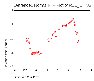
Figure 3: Comparison of detrended
cumulative probability with a normal distribution
This figures shows the
representation of relative change for household water demand for the Fairlight
region. If the relative changes were normally distributed, the dots would be
plotted alongside the horizontal line.
As the tests undertaken tend to
confirm the assumption that this sample does not suit a normal pattern, further
analysis indicate that the property shown, a relatively fat tail, and thin
peak, is known as leptokurtosis.
Failing to use normal
distributions, even with time-dependent mean and variance considered by
economists, physicists like Per Bak (Bak 1997)
used the power law devised by Pareto in 1893. If the data observed suit this
kind of distribution, the consequences are important. The probability density
function of the pareto distribution has two parameters, one, a, as the peakedness parameter, in the interval (0,2], and the other, b, as the skewness parameter, in the interval [-1,1]. The issue is that
these parameters have critical values. When a is equal to 2, the characteristic function of the paretian distribution
reduces to that of the normal distribution. But for a < 2, there is no finite variance for the distribution, and for a less or equal to 1, there is no finite mean.
Moss (2001) has investigated the
different means to generate such a distribution. The three mutually exclusive
explanations are: a normal distribution with predictable time varying
parameters, a stable pareto distribution with infinite variance generated by
self organised critical social process, or a non stable distribution generated
by a self organised critical social process.
Self organised critical processes
can be generated by systems that present social embeddedness. It is defined in
Edmonds 1999, as “the extent to which modelling the behaviour of an agent
requires the inclusion of other agents as individuals rather than an
undifferentiated whole”. It means that formally, it is more relevant to model
an agent as a part of the total system of agents and their interactions as
opposed to modelling it as a single agent that is interacting with an
essentially unitary environment.
The classical statistical
approach used is parametric statistics. Another option is to use non
parametrics statistics. It cannot really be used for inference, as one cannot
actually provide a non parametric model for forecasting, but can be used
instead to characterise an already existing data sample.
But as seen earlier, this
assumption does not always hold, and as it is likely the case now. Because the
assumptions required to use parametric statistics are at most debatable in the
current case, it puts the reliability, hence the utility of standard methods in
jeopardy.
What can then be used to analyse
the samples are nonparametric methods. Also be called “distribution-free”
methods, they do not assume the underlying distribution of the variable
involved, and consequently, none of their eventual properties. Instead, they
are based on ordinal measurements. Consequently, while the nonparametric
methods are not as powerful as parametric ones when in the correct situation,
they are much more powerful in cases such as this one when data cannot be
assumed to be normal).
The overall principle of the
nonparametric methods used in this research is that a sample can be compared to
another by verifying whether the distribution of their variations is either
consistent with a know distribution (that method is used to demonstrate that
the data, both observed and generated, are unlikely to match normality
assumptions), or similar to one another (that is used to demonstrate that the
results obtained by multiple simulations have the same underlying distribution,
and that this distribution can be considered as matching the observed data).
The use of MAS and the resulting model
The research into climate change
issues and the impact upon household water demand has led to the generation of
a model, using Integrated Assessment (Moss, 2001). Multi disciplinary inputs
have helped to make the representation as sensible as possible, and multi agent
systems were used, in order to represent the behaviour of households in terms
of water demand. It is devised as a dynamic representation of a society
composed of reactive agents (Ferber, 1999) influenced by their environment,
both social and physical.
The model used is based on Moss
and al. (2000) and Barthélémy and al. (2002). It incorporates agents
representing several households and a policy agent. The households are
characterised by their location on a grid, and a set of ownership, volume per
use, and frequency of use of appliances. The households can observe and
evaluate subjectively their neighbours, their activities, and the appliances. They
can therefore rate differently the information depending on its source.
The policy agent reacts to the
climatic conditions, and broadcasts messages of water saving in case of
dryness. Innovation is also present, as some appliances can break down, and be
replaced by newly available substitutes with different characteristics.
Amongst the processes embedded in
the model, a particular attention is given to the influence of innovation, its
presence and diffusion, as well as the importance of population response to the
various signals, from the policy agent or the neighbouring households.
The outputs of such simulations
can either be a straightforward analysis of the water demand generated by the
simulated households, or a more qualitative analysis of a specific phenomenon,
or of the characteristics or patterns (rather than the values themselves) of
the water demand. The latter will have our attention, that’s why it is
necessary to present the few assumptions that were found or thought to be of
importance in the model.
Some formal models are simple
enough so that the few parameters are meaningful ones with respect to the
object of the modelling. It is for example the case when dealing with the
evaluation of weight category for a person with respect to current weight and
physical characteristics. There are more complex models, for which the
sophistication requires many aspects of a problem to be taken into account. It
is then possible that some parameters integrated to the model could influence
significantly the results, while not being central to the modeller. Based on
simple model, Hales and Edmonds (2003) have given an example of modelling
details that, although not really central to their issue, turned out to be
decisive for the behaviour of the model, and the observed phenomenon.
During the verification and
validation processes, several particularities have been observed. The first one
refers to the innovation process, and the diffusion of new technologies. The
second one refers to the importance of initial conditions, and the way they are
implemented into the model.
In
Duboz et al. (2001) for example, the Multi
agent system used is tested for boundary conditions, i.e. a change in the
algorithms that are involved in the spatial behaviour of agents (namely the way
the agent bounces off a wall). Are also tested the distribution algorithms and
the size of the space, and the conclusion suggests that the choice of the
bouncing algorithm is a more important parameter than the distribution or size
of the population of agents.
In the current case, there are
many parameters and algorithms. The methods and values used are carefully
selected as having appropriate characteristics and (in general a lack of)
underlying assumptions.
Innovation
Quite an exhaustive view of
innovation diffusion can be found in (Rogers Everett 1995). He defines diffusion as “the process by which an innovation is
communicated through certain channels over time among the members of a social
system”.
Rogers presents all (or nearly)
the aspects of innovation, from its generation to its consequences, through the
study of its diffusion through the characteristics of the technology, of the
user, and of the underlying network. It is noticeable that the diffusion of
innovation depends then a lot on the nature of the innovation. They have
specific characteristics that could explain the rate of adoption, i.e. the
success or the failure of a given technology: relative advantage,
compatibility, complexity, trialability, and observability. Some even display
self-reinforced dynamics, when the technology can benefit from network
externalities. What is taken in to account then is the global influence of the
number of adopters in the system, not only locally (Blume [1993], Ellison
[1993]).
These characteristics are obviously
tightly depending on the technology itself and hence will not be included
extensively in the present study for the aforementioned reasons. The common
literature, mainly composed of surveys, is globally presenting these
characteristics of the technology along with the characteristics of the
individuals to explain the success or failure of some specific cases.
After many studies and debates, a scale and
a classification appeared. Proposed by Rogers in 1962, it is based on the
assumption that the frequency of adoption follows a bell-shaped curve, and the
associated cumulative curve is S-shaped. The adopters are then categorised
depending on their time of adoption.
·
The innovators are the first 2.5%
·
The early adopters are the next 13.5%
·
The early majority is the next 34%
·
The late majority is the next 34%
·
The laggards are the last 16%
These numbers are based on the
intervals each side of the average time of adoption. The innovators are more
than 2 standard deviations less than the average, while it is only one for
early adopters, the early majority is situated within a standard deviation less
than the average, the late majority is within a standard deviation more than
the average, and the laggards are adopting a technology after a period of time
that is more than the average plus one standard deviation. Trondsen (1996),
Valente (1996) and Young (2002) amongst others refer to these values, and
present results that conform to these categories.
One of the issues with such a
theory s that one cannot know beforehand which agent is which, unless the size
of the market is known in advance. It then becomes impossible to use this
approach in order to represent the diffusion of innovation in markets that
could be smaller than the whole population. In this model, the adoption process
for innovation is based on endorsements. In this matter, one can argue that the
subjectivity of the indicator selected can be such that it will direct the
whole pattern of adoption.
It was seen though that with this
particular type of representation, when the choice had to be made at random,
the bell-shaped pattern emerged in multiple occasions.
Technically, the reason for this
random selection is that amongst the endorsements recalled by the agent in
order to assess their values and select the highest, most of them were
equivalent. In certain cases, an agent looked for a specific type of
endorsement, and could not find them. It was then automatically considering
every endorsement value as zero.
Initial conditions
The initial conditions for this
model are based upon real life observation, and research upon the assumptions
made in the different scenarios generated by the Environment Agency.
Amongst the various assumptions,
three are of importance in this context.
- The representation of social values for every
scenario
The representation of the social
values of households does not imply anything in terms of the modelling of the
structures and the environment. The implications are concerning the way they
see and judge that environment. The argument here is that someone caring about
community will put a greater emphasis on the community as a driver of his own
behaviour. Selecting the appropriate weights of influence in the already
existing model can then represent this indicator. The endorsements can be
ranked, from an individualistic (self centred) point of view, to a more citizen
(globally influenced). They can therefore be used to represent the concern, and
influence, of a particular agent. The link is made here between the fact that
an agent is community oriented, and its major influences are in the “community”
around him, his neighbourhood. Nevertheless, while is easier to argue that
individualism can be linked with the references in the model to the
self-centred beliefs and rules, community can be a bit more difficult in the
framework of this model. What is called community in the EA approach is
actually referred as “community” within the model as the immediate social
environment of the agent. As it is expressed in their description, community
also seems to have the meaning of “citizenship”, a behaviour in line with the
idea of not wasting limited resources.
- The representation of the governance structure
through the distinctive characteristics of the scenarios
While the social values can be
represented in such a way that various ones can be generated easily, through a
simple choice of different ranking and / or values of the endorsements
themselves, it is not possible for the governance structure. As expressed
earlier, there are issues with the meaning of such an indicator, that prevent
from implementing it in a single and specific way. Consequently, unlike the
first part of the influences, this classification of the scenarios will be done
using the detailed approach. For a given state of social values, the governance
structure will be identified (and the scenario defined) by the range of
available appliances, their associated values (ownership, frequency, volume,
replacement rate), as well as the presence or not of technological regulations.
- The representation of the regulator through
the availability of resource saving appliances.
The representation of the
technological regulator is simple. Since the regulations are enforced in the
scenarios, there is no need for a dynamic adaptive regulation, i.e. the presence
in the model of an agent that would evaluate the situation and eventually
decide for the need of intervention. Like the emergence of new appliances,
which was already implemented, it is present as a constraint upon the
appliances. Since the scenarios describe accurately when regulation happens,
the influence on the model is that from a given date onwards, some devices are
made available, or unavailable for the households.
The layout of the support for the
agents can be important, and slightly different properties generate different
outcomes. In this case, the agents are situated on a regular grid limits. What
has been investigated though, is the impact of the grid structure itself. It
can be considered as a bidimensional mapping, or a tridimensional mapping, the
latter being equivalent to a toroidal shape, allowing agents to observe more
cells when they are located towards the edge of the grid.
The study of both situations
tends to show that although there is a significant difference in the links between
agents, it does not seem to generate large differences in the behaviours. It
can be assimilated to an increased possibility of communication amongst the
agents.
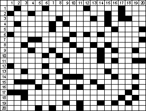
Fig 4: Matrix of links for a grid with a toroidal
structure: in this case, the 20 agents are situated on a grid of size 8*8.
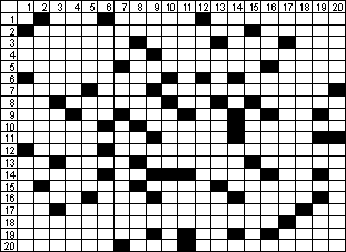
Fig 5: The equivalent matrix of links for the
non-toroidal version can be displayed as follow:
Since the black cells show the
existence of an interaction between the agents listed horizontally and
vertically, it is easy to notice that the toroidal structure provides more
contacts to each agent.
A significant difference could
not be proven to result from such changes, as long as the situations were
similar enough (i.e. there were not multiple simultaneous parameter changes).
Nevertheless, their influence
upon the results of the model needs to be understood, in order to improve the
model’s comprehension.
Algorithm used
While using power law distributed frequency and volumes
for the agents, some peaks of consumption appeared in the outputs. They were
initially though to be caused by drought periods, since the model is devised to
capture this process. Despite this, the fact that some peaks did not seem to
correspond to dry periods lead to a more thorough investigation of all peaks.
The outcome was actually that the particular implementation of the model
allowed in some rare cases the agent representing the institutions to broadcast
a message encouraging households to use more water than they were.
This phenomenon does not appear
in the alternative, where the frequency and volume are normally distributed,
but then it does not result in satisfactory outcomes.
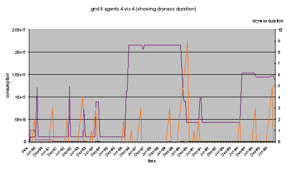
Fig 6: Peaks in demand observed
in parallel with dryness duration in the model
One could expect that the effect
of dryness would drive consumption down. The matching of these visual
indications reveals that the reaction to an exhortation from the policy agent
is not always producing the expected effect. Only the major dryness period
lasting for 9 months 1991 had an important and significant effect upon the
water consumption (as well as the subsequent ones, but on a smaller scale). The
other dryness periods actually seem to have no effect while only when the level
is already very high, a decrease can be observed.
This demonstrates that either the
behaviour of the agents is not implemented properly, or that there can be other
method related issues.
Although this behaviour does not
seem to affect the vast majority of the runs, it requires investigation to
understand what is the cause of such variance within the simulations.
The detailed study of this run
shows exactly what is happening. As expressed in the description of the model,
the policy agent uses a kind of average of the observed frequency and volume
data from the households. Due to the initial conditions, the policy agent could
then be biased by some extreme randomised value for the households.
It would therefore broadcast a
message that would lead households to adapt by using patterns whose recommended
values are higher than those in use by the households themselves.
Also, as one would expect, the
different cases of population repartition show that the favourable repartition
of the population towards agents that are marginally influenced by their
environment tend to generate patterns with significantly higher water demand
levels. That could be explained by the shift of influence from a
citizen-centred view to a more self centred one. One could then consider that
the messages from the institutions are not rated high enough to result in a
change of behaviour from the households.
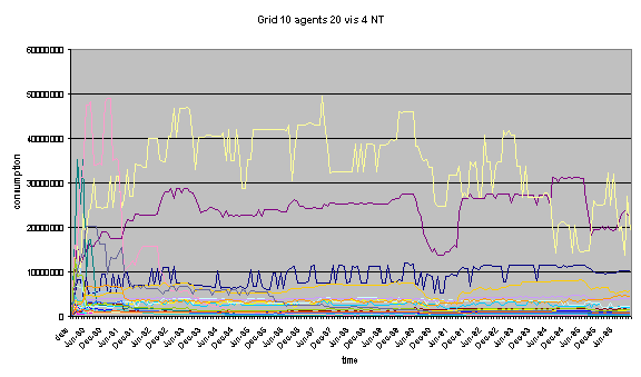
Finally, the global demand for water generated by a
set of runs for this model can be displayed as follows:
Fig 7: Chart of multiple runs for
the same simulation settings
This shows the evolution of water
demand for the entire population, i.e. 20 agents in this case, which are
located on a grid of size 10, on which they can see what their neighbours are
doing up to 4 cells away, without being limited by the edge of the grid.
Due to the unavoidable (at this
stage) effects of the power law implementation, some of the runs are not likely
to be representative of a standard behaviour. Still, the majority of the runs
are similar and could certainly be considered as representative of a scenario.
Conclusion
As a model is devised to analyse
the multiple issues surrounding the use of scenarios describing plausible
futures, the multi agent system used demonstrates the importance of careful
implementation of objects and processes.
The multi agent system can generate
patterns that are consistent, and that seem more accurate on a statistical
point of view than the traditional parametric approaches used in other studies
on the same subject.
While generally the sensitivity
to the initial conditions is investigated, it is found that sometimes, trivial
choices of modelling, or even coding, can have an important impact upon the
validity of the model itself.
During the course of the
validation and verification processes, interesting phenomenon could be
identified, and demonstrated some interesting properties. Further investigation
will be necessary in order to improve
the understanding of the reasons for this surprising diffusion process, as well
trying to avoid the emergence of extreme scenarios.
References:
Bak, P., 1997, How Nature Works: The Science of Self Organized
Criticality (Oxford, Oxford University Press).
Barthélémy O. Moss S., Downing T., Rouchier J., (2002), Policy Modelling
with ABSS: The Case of Water Demand Management, CPM report 02-92
R. Duboz, E. Ramat and P. Preux, Towards a coupling of continuous and
discrete formalisms in ecological
modelling - influences of the choice of algorithms on results, In proceedings
of the 13th European Symposium on Simulation, Marseille 10/18/2001-10/20/2001
(p481-487).
Edmonds, B. (1999). Capturing Social Embeddedness: a Constructivist
Approach. Adaptive Behavior, 7:323-348
Environment Agency, 2001, A scenario Approach to water demand
forecasting, Environment Agency
Ferber J., 1999, Multi-Agent Systems: An Introduction to Distributed
Artificial Intelligence, Addison-Wesley Edmonds B, Hales D, M2M Communication,
2003
Hales D, Edmonds, B, 2003, M2M conference,
Marseille, 31/03-01/04/2003
Herrington, P. and E. (1996). Climate change and the demand for water.
London, Hmso 1996.
Jensen, H., 1998, Self-Organized Criticality: Emergent Complex Behaviour
in Physical and Biological Systems (Cambridge: Cambridge University Press).
Moss, S., 2000, Competition in Intermediated markets: statistical
signatures and critical densities, CPM Report 01-79
Moss S., Downing T., Rouchier J., 2000, Demonstrating the Role of
Stakeholder Participation: An Agent Based Social Simulation Model of Water
Demand Policy and Response, CPM Report 00-76
Moss, S., Pahl-Wostl, C. and Downing, T., "Agent based integrated
assessment modelling", Integrated Assessment 2: 17-34, 2001
Rogers Everett, M. (1995). Diffusion of innovations. New York ; London,
Free Press.
Trondsen T.J., 1996, Some characteristics of adopters of a major
innovation in the computer field and its potential use in marketing, INDUSTRIAL
MARKETING MANAGEMENT, vol. 25, issue 6.
Valente T.W., 1996, Social Networks thresholds in the diffusion of
innovation, Social Networks, vol. 18, pp. 69-89.
Young, P.H. 2002, The diffusion of innovation in social networks,
working paper, The Santa Fe Institute