1. Introduction: Towards A Cognitive
Game Theory
Conflicts
as diverse as those between neighbors, friends, business associates, ethnic
groups, or states, often ensue from the same fundamental logic. On the one hand
the parties involved have common interests, such as avoidance of an all out
nuclear war, on the other hand they may fall prey to the temptation to pursue individual
agendas at the expense of the commons. To explore how and under what conditions
such relationships may proceed cooperatively rather than conflictuous, game
theory formalizes the problem of cooperation. At the
most elementary level, the theory represents relationships as a mixed-motive
two-person game with two choices, cooperate and defect. These choices intersect
at four possible outcomes, abbreviated as CC,
CD, DD, and DC. Each outcome
has an associated payoff: R (reward),
S (sucker), P (punishment) and T
(temptation), respectively. Using these payoffs, we define a two-person social
dilemma[1]
as any ordering of these payoffs such that mutual cooperation is Pareto optimal
yet may be undermined by the temptation to cheat (if T>R) or by the fear of
being cheated (if P>S) or by both. In the game of “Stag
Hunt” the problem is “fear” but not “greed” (R>T>P>S),
and in the game of “Chicken” the problem is “greed” but not “fear” (T>R>S>P).
The problem is most challenging when both fear and greed are present, that is,
when T>R and P>S. Given the assumption that R>P, there is only one way this can
happen, if T>R>P>S, the
celebrated game of “Prisoner’s Dilemma” (PD).
The Nash equilibrium[2] - the main solution concept in analytical game theory - predicts mutual defection in PD, unilateral defection in Chicken, and either mutual cooperation or mutual defection in Stag Hunt. However, Nash cannot make precise predictions about the selection of supergame equilibria, that is, about the outcome of on-going mixed-motive games. Nor can it tell us much about the dynamics by which a population of players can move from one equilibrium to another. These limitations, along with concerns about the cognitive demands of forward-looking rationality (Dawes and Thaler 1988; Weibull 1998; Fudenberg and Levine 1998), have led game theorists to explore models of cognition that explicitly describe the dynamics of stepwise decision making. This is reflected in a growing number of formal learning-theoretic models of cooperative behavior (Macy 1991; Roth and Erev 1995; Fudenberg and Levine 1998; Peyton-Young 1998; Cohen et. al. 2001). In learning, positive outcomes increase the probability that the associated behavior will be repeated, while negative outcomes reduce it.
In general form, these simple game-theoretic learning models consist of a probabilistic decision rule and a learning algorithm in which game payoffs are evaluated relative to an aspiration level, and the corresponding choice propensities are updated accordingly. The schematic model is diagrammed in Figure 1.
Figure 1. Schematic model of reinforcement learning.
The first step in Figure 1 is the decision by each player whether to cooperate or defect. This decision is probabilistic, based on the player’s current propensity to cooperate. The resulting outcome then generates payoffs (R, S, P, or T) that the players evaluate as satisfactory or unsatisfactory relative to their aspiration level. Satisfactory payoffs present a positive stimulus (or reward) and unsatisfactory payoffs present a negative stimulus (or punishment). These rewards and punishments then modify the probability of repeating the associated choice, such that satisfactory choices become more likely to be repeated, while unsatisfactory choices become less likely.
Erev, Roth and others
(Roth and Erev 1995; Erev and Roth 1998; Erev et al. 1999) used a learning model to estimate globally
applicable parameters from data collected across a variety of human subject
experiments. They concluded that “low rationality” models of reinforcement learning
may often provide a more accurate prediction than orthodox game theoretical
analysis. Macy (1995) and Flache (1996) have also tested a simple reinforcement
learning algorithm in controlled social dilemma experiments and found supporting
evidence.
Learning models have
also been applied outside the laboratory to mixed-motive games played in
everyday life, in which cooperation is largely unthinking and automatic, based
on heuristics, habits, routines, or norms, such as the propensity to loan a
tool to a neighbor, tell the truth, or trouble oneself to vote. For example,
Kanazawa (2000) used voting data to show how a simple learning model suggested
by Macy (1991) solves the “voter paradox” in public choice theory.
While interest in cognitive game theory is clearly growing, recent studies have been divided by disciplinary boundaries between sociology, psychology, and economics that have obstructed the theoretical integration needed to isolate and identify the learning principles that underlie new solution concepts. Our paper aims to move towards such an integration. We align two prominent models in cognitive game theory and integrate them into a general model of adaptive behavior in two-person mixed-motive games (or social dilemmas). In doing so, we will identify a set of model-independent learning principles that are necessary and sufficient to generate cooperative solutions. We begin by briefly summarizing the basic principles of reinforcement learning and then introduce two formal specifications of these principles, the Bush-Mosteller stochastic learning model and the Roth-Erev payoff matching model.
1.1 Learning Theory and the Law of Effect
In
reinforcement learning theory, the search for solutions is “backward-looking”
(Macy 1990) in that it is driven by experience rather than the forward-looking
calculation assumed in analytical game theory (Fudenberg and Levine 1998;
Weibull 1998). Thorndike (1898) formulated this as the “Law of Effect,” based
on the cognitive psychology of William James. If a behavioral response has a
favorable outcome, the neural pathways that triggered the behavior are
strengthened, which “loads the dice in favor of those of its performances which
make for the most permanent interests of the brain’s owner” (James 1981, p.
143). This connectionist theory anticipates the error back-propagation used in
contemporary neural networks (Rummelhart and McLelland 1988). These models show
how highly complex behavioral responses can be acquired through repeated
exposure to a problem. For example, with a little genetic predisposition and a
lot of practice, we can learn to catch a ball while running at full speed,
without having to stop and calculate the trajectory (as the ball passes
overhead).
More
precisely, learning theory relaxes three key behavioral assumptions in
analytical game-theoretic models of decision:
·
Propinquity replaces causality as the link between choices
and payoffs. Learning theory
assumes experiential induction rather than logical deduction. Players explore
the likely consequences of alternative choices and develop preferences for
those associated with better outcomes, even though the association may be
coincident, “superstitious,” or causally spurious.
·
Reward and punishment replace utility as the motivation for
choice. Learning theory differs
from game-theoretic utility theory in positing two distinct cognitive
mechanisms that guide decisions toward better outcomes, approach (driven by reward) and avoidance
(driven by punishment). The distinction means that aspiration levels are
very important for learning theory. The effect of an outcome depends decisively
on whether it is coded as gain or loss, satisfactory or unsatisfactory,
pleasant or aversive.
·
Melioration
replaces optimization as the basis for the distribution of choices over time. Melioration refers to suboptimal gradient climbing when confronted
with “distributed choice” (Herrnstein and Drazin 1991) across recurrent
decisions. Melioration implies a tendency to repeat choices with satisfactory
outcomes even if other choices have higher utility, a behavioral tendency March
and Simon (1958) call “satisficing.” In contrast, unsatisfactory outcomes
induce search for alternative outcomes, including a tendency to revisit
alternative choices whose outcomes are even worse, a pattern we call
“dissatisficing.”
The
Law of Effect does not solve the social dilemma, it merely reframes it: Where the penalty for cooperation is larger
than the reward, and the reward for aggressive behavior is larger than the
penalty, how can penalty-aversive, reward-seeking actors elude the trap of
mutual punishment?
1.2 The Bush-Mosteller Stochastic Learning Model
The earliest answer was given by Rapoport and Chammah (1965), who used learning theory to propose a Markov model of Prisoner’s Dilemma with state transition probabilities given by the payoffs for each state, based on the assumption that each player is satisfied only when the partner cooperates. With choice probabilities updated after each move based on the Law of Effect, mutual cooperation is an absorbing state in the Markov chain.
Macy (1990, 1991)
elaborated Rapoport and Chammah’s analysis using computer simulations of their
Bush-Mosteller stochastic learning model. Macy identified two
learning-theoretic equilibria in the PD game, corresponding to each of the two
learning mechanisms, approach and avoidance. Approach implies a
self-reinforcing equilibrium (SRE)
characterized by satisficing behavior. The SRE obtains when a strategy pair
yields payoffs that are mutually rewarding. The SRE can obtain even when both
players receive less than their optimal payoff (such as the R payoff for mutual cooperation in the
PD game), so long as this payoff exceeds aspirations. Avoidance implies an
aversive self-correcting equilibrium (SCE) characterized by dissatisficing
behavior. Dissatisficing means that both players will try to avoid an outcome
that is better than their worst possible payoff (such as P in the PD game), so long as this payoff is below aspirations. The
SCE obtains when the expected change of probabilities is zero and there is a
positive probability of punishment as well as reward. This happens when
outcomes that reward cooperation or punish defection (causing the probability
of cooperation to increase) balance outcomes that punish cooperation or reward
defection (causing the probability to decline).[3] At equilibrium,
the dynamics pushing the probability higher are balanced by the dynamics
pushing in the other direction, like a tug-of-war between two equally strong
teams.
These learning
theoretic equilibria differ fundamentally from the Nash predictions in that
agents have an incentive to unilaterally change strategy. In the SRE, both
players have an incentive to deviate from unconditional mutual cooperation, but
they stay the course so long as the R
payoff exceeds their aspirations. Unlike the Nash equilibrium, the SCE has
players constantly changing course, but their efforts are self-defeating. It is
not that everyone decides they are doing the best they can, it is that their
efforts to do better set into motion a dynamic that pulls the rug out from
under everyone.
Suppose two players in
PD are each satisfied only when the partner cooperates, and each starts out
with zero probability of cooperation. They are both certain to defect, which
then causes both probabilities to increase (as an avoidance response).
Paradoxically, an increased probability of cooperation now makes a unilateral
outcome (CD or DC) more likely
than before, and these outcomes punish the cooperator and reward the defector,
causing both probabilities to drop. Nevertheless, there is always the chance
that both players will defect anyway, causing probabilities to rise further
still. Once both probabilities exceed 0.5, further increases become
self-reinforcing, by increasing the chances for another bilateral move, and
this move is now more likely to be mutual cooperation instead of mutual
defection. In short, the players can escape the social trap through stochastic collusion, characterized by a
chance sequence of bilateral moves in a “drunkard’s walk.” A fortuitous string
of bilateral outcomes can increase cooperative probabilities to the point that
cooperation becomes self-sustaining - the drunkard wanders out of the gully.
1.3 The Roth-Erev Payoff-Matching Model
More
recently, Roth and Erev (Roth and Erev 1995; Erev and Roth 1998; Erev et al.
1999) have proposed a learning-theoretic alternative to the earlier
Bush-Mosteller formulation. Their model draws on the “matching law” which holds
that adaptive actors will choose between alternatives in a ratio that matches
the ratio of reward. Applied to social dilemmas, the matching law predicts that
players will learn to cooperate to the extent that the payoff for cooperation
exceeds that for defection, which is possible only if both players happen to
cooperate and defect at the same time (given R>P). As with
Bush-Mosteller, the path to cooperation is a sequence of bilateral moves.
Like the Bush-Mosteller
stochastic learning model, the Roth-Erev payoff matching model implements the three
basic principles that distinguish learning from utility theory – experiential
induction (vs. logical deduction), reward and punishment (vs. utility), and
melioration (vs. optimization). The similarity in substantive assumptions makes
it tempting to assume that the two models are mathematically equivalent, or if
not, that they nevertheless give equivalent solutions.
On closer inspection,
however, we find important differences. Each specification implements
reinforcement learning in different ways, and with different results. Without a
systematic theoretical alignment and integration of the two algorithms, it is
not clear whether and under what conditions the backward-looking solution for
social dilemmas identified with the Bush-Mosteller (BM) specification generalizes
to the Roth-Erev (RE) model.
Those assumptions can
be brought to the surface by close comparison of competing models and by
integrating alternative specifications as special cases of a more general
model. This is especially important for models that must rely on computational
rather than mathematical methods. “Without such a process of close comparison,
computational modeling will never provide the clear sense of ‘domain of
validity’ that typically can be obtained for mathematized theories” (Axtell et
al. 1996, p. 123).
Unfortunately, learning
models have been divided by disciplinary boundaries between sociology,
psychology, and economics that have obstructed the theoretical integration
needed to isolate and identify the learning principles that underlie new
solution concepts. Accordingly, this paper aims to align two prominent models
in cognitive game theory and to integrate them into a general model of adaptive
behavior in two-person mixed-motive games. By “docking” (Axtell et al. 1996)
the BM stochastic learning model with the RE payoff-matching model, we can
identify learning principles that generalize beyond particular specifications,
and at the same time, uncover hidden assumptions that explain differences in
the outcomes and constrain the generality of the theoretical derivations.
In section 2 that
follows, we formally align the two learning models and integrate them into a
General Reinforcement Learning (GRL) model, for which the Bush-Mosteller and
Roth-Erev models are special cases. This process brings to the surface a key
hidden assumption with important implications for the generality of
learning-theoretic solution concepts. Section 3 then uses computer simulations
of the integrated model to explore the effects of model differences across a
range of two-person social dilemma games. The analyses confirm the generality
of stochastic collusion but also show that its determinants depend decisively
on whether BM or RE assumptions about learning dynamics are employed.
2. The Bush-Mosteller and Roth-Erev
Specifications
In general form,
both the BM and RE models implement the stochastic decision process diagrammed
in Figure 1, in which choice propensities are updated by the associated
outcomes. Thus, both
models imply the existence of some aspiration level relative to which cardinal
payoffs can be positively or negatively evaluated. Formally, the stimulus s associated with action a is calculated as
![]() [1]
[1]
where
pa is the payoff
associated with action a (R or S
if a = C, and T or P if a = D) and sa is a positive or negative stimulus derived from pa. The denominator in [1] represents the upper value of the
set of possible differences between payoff and aspiration. With this scaling
factor, stimulus s is always equal to
or less than unity in absolute value, regardless of the magnitude of the corresponding
payoff.[4]
Neither model
imposes constraints on the determinants of aspirations.
Whether aspirations are high or low or
habituate with experience depends on assumptions that are exogenous to both
models.
2.1 Aligning the two models
The
two models diverge at the point that these evaluations are used to update
choice probabilities. The Bush-Mosteller stochastic learning algorithm updates
probabilities following an action a
(cooperation or defection) as follows:
 [2]
[2]
In
equation [2], pa,t is the
probability of action a at time t and ![]() is the positive
or negative stimulus given by [1]. The change in the probability for the action
not taken, b, obtains from the
constraint that probabilities always sum to one, i.e.
is the positive
or negative stimulus given by [1]. The change in the probability for the action
not taken, b, obtains from the
constraint that probabilities always sum to one, i.e. ![]() . The parameter l
is a constant (0 < l < 1) that
scales the learning rate. With l » 0, learning is
very slow, and with l » 1,
the model approximates a “win-stay, lose-shift” strategy (Catania 1992).
. The parameter l
is a constant (0 < l < 1) that
scales the learning rate. With l » 0, learning is
very slow, and with l » 1,
the model approximates a “win-stay, lose-shift” strategy (Catania 1992).
For any value of l, Equation 2 implies a decreasing
effect of reward as the associated propensity approaches unity, but an
increasing effect of punishment. Similarly, as the propensity approaches zero,
there is a decreasing effect of punishment and a growing effect of reward. This
constrains probabilities to approach asymptotically their natural limits.
Like the
Bush-Mosteller, the Roth-Erev model is stochastic, but the probabilities are
not equivalent to propensities. Propensities are a function of cumulative
satisfication and dissatisfaction with the associated choices, and
probabilities are a function of the ratio of propensities. More precisely, the
propensity q for action a at time T is the sum of all stimuli ![]() a player has ever
received when playing a:
a player has ever
received when playing a:
![]() [3]
[3]
Roth and Erev then use a “probabilistic choice rule” to
translate propensities into behavior. The probability pa of action a
at time t+1 is the propensity for a divided by the sum of the propensities
at time t:
![]() [4]
[4]
where
a and b represent the binary choices to cooperate or defect. Following
action a, the associated propensity qa increases if the payoff is
positive relative to aspirations (by increasing the numerator in [4]) and
decreases if negative. The propensity for b
remains constant, but the probability of b
declines (by increasing the denominator in the equivalent expression for pb,t+1).
An obvious problem with
the specification of equations [3] and [4] (but not [2]) is the possibility of
negative probabilities if punishment dominates reinforcement. In their original
model, Erev, Roth and Bereby-Meyer (1999) circumvent this problem with the ad hoc addition of a “clipping” rule.
More precisely, their implementation assumes that the new propensity qa,t+1 = qa,t + sa,t except for
the case where this sum drops below a very small positive constant n. In that case, the
new propensity is reset to n. Equations [5] and [6] represent the RE
clipping rule by rewriting [3] as
![]() [5]
[5]
where
a is the action taken in round t (either cooperation or defection) and r is a response function of the form
 [6]
[6]
where
all terms except n are indexed on t.
This solution causes the response to reinforcement to become discontinuous as
propensities approach the lower bound n. In order to align the model with
Bush-Mosteller, we replaced the discontinuous function in [6] with a more
elegant solution. Equation [7] gives asymptotic lower as well as upper limits
to the probabilites:
 [7]
[7]
where
all terms except l (the constant
learning rate) are indexed on t. The
parameter l sets the baseline
learning rate between zero and one (as in [2]), rather than leaving l implied by the relative magnitude of
the payoffs (as in [3]). More importantly, [7] aligns Roth-Erev with
Bush-Mosteller by eliminating the need for a theoretically arbitrary clipping
rule. For sa ³ 0, [7] is
equivalent to [6] except that rewards are multiplied by the constant ![]() that increases exponentially
with the learning rate l. The
important change is for the case where sa
< 0. Now r is decreasing in qa (with a limit at zero).
Hence, the marginal effect of additional punishment for action a approaches zero as the corresponding
propensity approaches zero.
that increases exponentially
with the learning rate l. The
important change is for the case where sa
< 0. Now r is decreasing in qa (with a limit at zero).
Hence, the marginal effect of additional punishment for action a approaches zero as the corresponding
propensity approaches zero.
Equation [7] aligns Roth-Erev with Bush-Mosteller,
allowing easy identification of the essential difference, which is inscribed in
equation [4]. Rewards increase the denominator in [4], depressesing the effect
on probabilities of unit changes in the numerator. Punishments have the
opposite effect, allowing faster changes in probabilities.
To see the significance
of this difference, consider first the special case where learning is based on
rewards of different magnitude and no stimuli are aversive. Here the RE model
corresponds to Blackburn’s (1936) "Power Law of Practice.” Erev and Roth
(1998) cite Blackburn to support the version of their model that precludes punishment,
such that “learning curves tend to be steep initially and then flatten"
(1998:859). In the version with both reward and punishment, their model implies
what might be termed a “Power Law of Learning,” in which responsiveness to
stimuli declines exponentially with reward and increases with punishment. We
have no knowledge of a Power Law of Learning or of any corresponding
learning-theoretic concept. For convenience, we have borrowed “fixation” from
Freudian psychology.
Fixation is the
principal difference between the BM and RE models. Unlike the BM model, which
precludes fixation, the RE model builds this in as a necessary implication of
the learning algorithm in [4]. The two models make convergent predictions
about:
- the declining marginal impact of
repeated reinforcement on the response to yet another reward.
- the increasing marginal impact of
repeated punishment on the response to an occasional reward.
However,
the two models make competing predictions about the effects of repeated
punishment on the response to additional punishment, and on the effects of
repeated reward on the response to an occasional punishment, as summarized in
Table 1. Bush-Mosteller assumes that the marginal impact of punishment
decreases with repetition, while punishment has its maximum effect following
repeated reward for a given action. The Power Law of Learning implies quite the
opposite. Repeated failure arouses attention and restores an interest in
learning. Hence, the marginal impact of punishment increases with punishment.
Conversely, repeated success leads to complacency and inattention to the
consequences of behavior, be it reward or punishment.
|
|
Following Repeated Reinforcement of C: |
Following Repeated Punishment of C: |
||||||
|
|
Response to
Reward |
Response to Punishment |
Response to
Reward |
Response to Punishment |
||||
|
|
of C |
of D |
of C |
of D |
of C |
of D |
of C |
of D |
|
BM |
Decreases |
Increases |
Increases |
Decreases |
Increases |
Decreases |
Decreases |
Increases |
|
RE |
Decreases |
Decreases |
Decreases |
Decreases |
Increases |
Increases |
Increases |
Increases |
Table 1. Change in response to reward and punishment following a
recurrent stimulus.
Note
that fixation as implemented in the RE learning model should not be confused
with either satisficing or habituation, two well-known behavioral mechanisms
that can also promote the routinization of behavior. Fixation differs from
satisficing in both the causes and effects. Satisficing is caused by a sequence
of reinforcements that are associated with a given behavior, which causes the
probability of choosing that behavior to approach unity, thereby precluding the
chance to find a better alternative. Fixation is caused by a sequence of
reinforcements for any behavior.
Thus, fixation “fixes” any probability distribution over a set of behaviors,
including indifference, so long as all behaviors are rewarded. Satisficing and
fixation also differ in their effects. Satisficing inhibits search but has no
effect on responsiveness to reinforcement. Fixation does not preclude search
but instead inhibits responses to the outcomes of all behaviors that may be
explored.
Fixation also differs
from habituation, in both the causes and effects. Habituation is caused by
repeated presentation of a stimulus, be it a reward or a punishment. Fixation
is caused only by repeated reinforcement; repeated punishment disrupts fixation
and restores learning. The effects also differ. Habituation to reward increases
sensitivity to punishment, while fixation inhibits responsiveness to both
reward and punishment.
2.2 Integrating the two models
To
suppress fixation, Roth and Erev (1995; see also Erev and Roth 1998) added
discontinuous functions for “forgetting,” which suddenly resets the propensity
to some lower value. Like the “clipping” rule, the “forgetting” rule is
theoretically ad hoc and
mathematically inelegant. Equation [8] offers a more elegant solution that
permits continuous variation in the level of fixation, parameterized as f:
 [8]
[8]
As
in [7], all parameters except f and l are time indexed. The parameter f represents the level of fixation,
0 £ f £ 1. Equation
[8] is identical to [7] in the limiting case where f = 1, corresponding to the RE model which fixation hardwired.
But notice what happens
when f = 0. Equation [8]
now reduces to the BM stochastic learning algorithm! (The
proof is elaborated in the Appendix.). By replacing the discontinuous “clipping” and “forgetting”
functions used by Roth-Erev with continuous functions, we arrive at a General
Reinforcement Learning (GRL) model, with a smoothed version of Roth-Erev and
the original Bush-Mosteller as special cases. Hence, the response function in
[8] is expressed as rG,
denoting the generality of the model. Bush-Mosteller and Roth-Erev are now
fully aligned and integrated.
3. A General Theory of Cooperation in
Social Dilemmas
The
GRL model in equations [1], [4], [5], and [8] includes three parameters - aspiration level (A), learning rate (l), and fixation (f) - that can be
manipulated to study each of the four mechanisms that we have identified as
elements of a learning-theoretic solution concept for social dilemmas:
satisficing, dissatisficing, fixation, and random walk.[5]
The model allows us to independently manipulate satisficing (precluded by high
aspirations), dissatisficing (precluded by low aspirations), fixation
(precluded by a fixed learning rate), and random walk (precluded by a low
learning rate). We can then systematically explore the solutions that emerge
with different parameter combinations over each of the three classic types of
social dilemma.
3.1 The Baseline Model: Stochastic Collusion in Social Dilemmas
We
begin by using the GRL model to replicate findings in previous research with
the BM specification. This provides a baseline for comparing the learning
dynamics in the RE model, specifically, the effects of fixation in interaction
with aspiration levels and learning rates.
Macy and Flache (2002)
used the BM model to study learning dynamics in three characteristic types of
two-person social dilemma games, PD, Chicken, and Stag Hunt. They idenfied a
socially deficient SCE in all three social dilemmas. We can compute SCE
analytically by finding the level of cooperation at which the expected change
in the probability of cooperation is zero. The expected change is zero when for
both players the probability of outcomes that reward cooperation or punish
defection, weighted by the absolute value of the associated stimuli, equals the
probability of outcomes that punish cooperation or reward defection, weighted
likewise. With A = 2 and
the payoff vector [4,3,1,0], the SCE occurs at pc = 0.37 in PD and at pc = 0.5 in Chicken and Stag Hunt,
respectively. Across all possible payoffs, the equilibrium cooperation rate in
PD is always below pc = 0.5,
which is the asymptotic upper bound that the solution approaches as R approaches T and P approaches S simultaneously. The lower bound is pc = 0 as P approaches A. In Chicken, the corresponding upper bound is pc = 1 as R approaches T and S approaches A. The lower bound is pc = 0 as R, S,
and P all converge on A (retaining R>A>S>P).
Only in Stag Hunt is it possible that there is no SCE, if R-T > A-S.
The lower bound for Stag Hunt is pc = 0
as T approaches R and P approaches A.
Using computer
simulation, Macy and Flache (2002) show that it is possible to escape this
equilibrium through random walk not only in Prisoner’s Dilemma but in all
dyadic social dilemma games. However, the viability of the solution critically
depends on actors’ aspiration levels, i.e. the benchmark that distinguishes
between satisfactory and unsatisfactory outcomes. A self-reinforcing
cooperative equilibrium is possible if and only if both players’ aspiration
levels are lower than the payoff for mutual cooperation (R). Aspirations above this point necessarily preclude a learning
theoretic solution to social dilemmas.
Very low aspirations do
not preclude mutual cooperation as an equilibrium but may prevent adaptive
actors from finding it. If aspiration levels are below maximin,[6]
then mutual or unilateral defection may also be a self-reinforcing equilibrium,
even though these outcomes are socially deficient. Once the two players stumble
into one of these outcomes, there is no escape, so long as the outcome is
mutually reinforcing. If the aspiration level exceeds maximin and falls below R, there is a unique SRE in which both players
receive a reward, namely, mutual cooperation.
If there is at least
one SRE in the game matrix, then escape from the SCE is inevitable. It is only
a matter of time until a chance sequence of moves causes players to lock-in a
mutually reinforcing combination of strategy choices. However, the wait may not
be practical in the intermediate term if the learning rate is very low. The
lower the learning rate, the larger the number of steps that must be
fortuitously coordinated to escape the “pull” of the SCE. Thus, the odds of
attaining lock-in increase with the step-size in a random walk (see also Macy
1989, 1991).
To summarize, the BM
stochastic learning model identifies a social trap - a socially deficient SCE - that lurks inside
every PD and Chicken game and most games of Stag Hunt. The model also
identifies a backward-looking solution, mutually reinforcing cooperation.
However, this solution obtains only when both players have aspiration levels
below R, such that each is satisfied
when the partner cooperates. Stochastic collusion via random walk is possible
only if aspirations are also above maximin and is viable for the intermediate
term only if the learning rate is sufficiently high.
We
can test whether these Bush-Mosteller results can be replicated with the GRL
model by setting parameters to preclude fixation and to allow random walk,
satisficing, and dissatisficing. More precisely:
·
Fixation is
precluded by setting f = 0.
·
Aspirations are
fixed midway between maximin and minimax. With the payoffs ordered from the set
[4,3,1,0] for each of the three social dilemma payoff inequalities, minimax is
always 3, maximin is always 1, and A = 2.
This aspiration level can be interpreted as the expected payoff when
behavioral propensities are uninformed by prior experience (pa = 0.5) such that all four
payoffs are equiprobable.This means that mutual cooperation is a unique SRE in
each of the three social dilemma games.
·
We set the
baseline learning rate l high enough
to facilitate random walk
into the SRE at CC (l = 0.5).
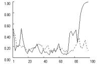
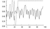
Figure
2 confirms the possibility of stochastic collusion in all three social dilemma
games, assuming moderate learning rates, moderate aspirations, and no fixation.
The figure charts the change in the probability of cooperation, pc for one of two players
with statistically identical probabilities.
|
|
|
|
|
Prisoner’s
Dilemma (T>R>A>P>S) |
Chicken (T>R>A>S>P) |
Stag Hunt (R>T>A>P>S) |
|
Figure 2.
Stochastic collusion in three social dilemma games. (p = [4,3,1,0], A = 2,
l = 0.5, f = 0, qc,1 = qd,1 = 1. |
||
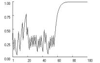
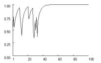
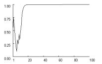
Figure 2 shows how
dissatisficing players wander about in a SCE with a positive probability of
cooperation that eventually allows them to escape the social trap by random
walk. With f = 0, the
general model reproduces the characteristic Bush-Mosteller pattern of
stochastic collusion in all three games, but not with equal probability. Mutual cooperation locks
in most readily in Stag Hunt and least readily in Prisoner’s Dilemma. To test
the robustness of this difference, we simulated 1000 replications of this
experiment and measured the proportion of runs that locked into mutual
cooperation within 250 iterations. The results confirm the differences between
the games. In Prisoner’s Dilemma, the lock-in rate for mutual cooperation was
only 0.66, while it was 0.96 in Chicken and 1.0 in Stag Hunt.
These differences
reflect subtle but important interactions between aspiration levels and the
type of social dilemma - the relative importance of fear (the problem in
Stag Hunt) and greed (the problem in Chicken). The simulations also show that
satisficing is equally important, at least in the Prisoner’s Dilemma and in the
Chicken Game. In these games, appreciation that the payoff for mutual
cooperation is “good enough” motivates players to stay the course despite the temptation
to cheat (given T>R). Otherwise, mutual cooperation will
not be self-reinforcing. In Stag Hunt, satisficing is less needed in the long
run, because there is no temptation to cheat (R>T). However, despite
the absence of greed, the simulations reveal that, even in Stag Hunt, fear may
inhibit stochastic collusion if high aspirations limit satisficing. Simulations
confirmed that, in the absence of fixation, there is an optimal balance point
for the aspiration level between satisficing and dissatisficing and between
maximin and R.
3.2 Effects of fixation on stochastic collusion
With
the Bush-Mosteller dynamics as a baseline, we now systematically explore the
effects of fixation in interaction with the learning rate and aspirations.
Knowledge of these effects will yield a general theory of the governing
dynamics for reinforcement learning in social dilemmas, of which BM and RE are
special cases.
Fixation has important
implications for the effective learning rate, which in turn influences the
coordination complexity of stochastic collusion. In both the BM and revised RE
models, the effective learning rate depends on the baseline rate (l) and the magnitude of p. Even if the baseline learning rate is
high, the effective rate approaches zero as p
asymptotically approaches the natural limits of probability. The RE model
adds fixation as an additional determinant of effective learning rates.
Fixation implies a tendency for learning to slow down with success, and this
can be expected to stabilize the SRE. Even if one player should occasionally
cheat, fixation prevents either side from paying much attention. Thus,
cooperative propensities remain high, and the rewards that induce fixation are
quickly restored.
Fixation also implies
that learning speeds up with failure. This should destabilize the SCE, leading
to a higher probability of random walk into stochastic collusion, all else
being equal. This effect of fixation should be even stronger when aspirations
are high. The higher actors’ aspirations, the smaller are the rewards and the
larger the punishments that players’ can experience. As aspirations approach
the R payoff (from below),
punishments may become so strong that “de-fixation” propels actors into
stochastic collusion following a single incidence of mutual defection.
The lower actors’
aspirations, the larger are the rewards and the smaller the punishments that
players’ can experience. Fixation on reward then reduces the effective learning
rate, thereby increasing the coordination complexity of random walk into the
SRE. The smaller the step size, the longer it takes for random walk out of the
SCE.
Simply put, when
aspirations are above maximin, the Power Law of Learning implies a higher likelihood
of obtaining a cooperative equilibrium in social dilemmas, compared to what
would be expected in the absence of a tendency toward fixation, all else being
equal. However, the opposite is the case when aspirations are low.
We used computational
experiments to test these intuitions about how fixation interacts with learning
rates and aspirations to alter the governing dynamics in each of three types of
social dilemma, using a two (learning rates: high/low) by two (fixation:
high/low) by two (aspirations: high/low) factorial design, with fixation and
aspiration levels nested within learning rates. Based on the results for the BM
model (with f = 0), we set the
learning rate l at a level high
enough to facilitate stochastic collusion (0.5) and low enough to preclude
stochastic collusion (0.05). We begin with a high learning rate in order to
study the effects of fixation on the attraction and stability of the SRE. We
then use a low learning rate to look at the effects on the stability of
socially deficient SCE.
Within each learning
rate, we manipulated fixation using two levels, f = 0, corresponding to the BM assumption and f = 0.5 as an approximation of the RE
model with a moderate level of fixation. (For robustness, we also tested f = 1 but found no qualitative
difference with moderate fixation.) Within each level of fixation, we
manipulated the aspiration level below and above A = 2.0 to see how fixation affects the optimal
aspiration level for random walk into mutual cooperation.
We begin by testing the
interaction between fixation and satisficing by setting aspirations close to
the lower limit at maximin. With A =
1.05 and l = 0.5, mutual
cooperation is the unique SRE in all three games, and stochastic collusion is
possible even without fixation. Low aspirations increase the tendency to
satisfice, making it more difficult to escape a socially deficient SCE. With
low aspirations, the predominance of reward over punishment means that fixation
can be expected to increase the difficulty by further stabilizing the SCE.
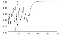
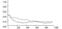
This intuition is
confirmed in Figure 3 across all three games. The dotted lines show the cooperation
rate with fixation (f = 0.5)
and the solid line shows the rate without fixation. Without fixation, low
aspirations delay lock-in on mutual cooperation relative to the moderate
aspirations in the baseline condition (see Figure 2), but lock-in is still
possible within the first 100 iterations. For reliability, we measured the
proportion of runs that locked in mutual cooperation within 250 iterations,
based on 1000 replications with A = 1.05.
We found that in the Prisoner’s Dilemma and in the Chicken Game, the lower
aspiration level caused a significant decline in the rate of mutual cooperation
relative to the baseline condition, but it did not suppress cooperation
entirely. In the Prisoner’s Dilemma, the cooperation rate declined from 0.66 in
the baseline condition to about 0.14, and for the Chicken Game the
corresponding reduction was from 0.96 to 0.83. Only in Stag Hunt did lower
aspirations not affect the rate of mutual cooperation.
|
|
|
|
|
Prisoner’s
Dilemma (T>R>A>P>S) |
Chicken (T>R>A>S>P) |
Stag Hunt (R>T>A>P>S) |
|
Figure 3.
Effect of low aspirations on cooperation rates, with and without fixation
(dotted and solid) in three social
dilemmas (p = [4,3,1,0], A = 1.05,
l = 0.5, f = [0, 0.5], qc,1 = qd,1 = 1). |
||
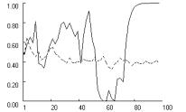
As
expected, fixation considerably exacerbates the problem caused by low
aspirations. Figure 3 shows how with f = 0.5,
lock-in fails to obtain entirely in the Prisoner’s Dilemma and Chicken, and is
significantly delayed in Stag Hunt. Reliability tests reveal a highly
significant effect of fixation. Based on 1000 replications with f = 0.5, the rate of lock-in
within 250 iterations dropped to zero in all three games.
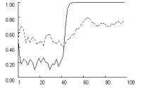
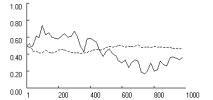
With high aspirations,
fixation should have the opposite effect. Without fixation, high aspirations
increase the tendency to dissatisfice (over-explore), which should destabilize
the SRE. However, the predominance of punishment over reward means that
“de-fixation” can be expected to promote cooperation by negating the
destabilizing effects of dissatisficing. This intuition is confirmed in Figure
4. For symmetry with Figure 3, we assumed an aspiration level of A = 2.95, just below the minimax payoff.
Without fixation, stochastic collusion remains possible but becomes much more
difficult to attain, due to the absence of satisficing.
|
|
|
|
|
Prisoner’s
Dilemma (T>R>A>P>S) |
Chicken (T>R>A>S>P) |
Stag Hunt (R>T>A>P>S) |
|
Figure 4.
Effect of high aspirations on cooperation rates, with and without fixation
(dotted and solid) in three social dilemmas (p = [4,3,1,0], A = 2.95,
l = 0.5, f = [0, 0.5], qc,1 = qd,1 = 1). |
||
Figure
4 reveals an effect of fixation that is similar across the three payoff
structures. Without fixation, high aspirations preclude stochastic collusion in
Prisoner’s Dilemma and Chicken. In Stag Hunt, mutual cooperation remains
possible but is delayed relative to the baseline condition in Figure 2. With
high aspirations, fixation causes the effective learning rate to increase
within the first 20 or so iterations, up to a level that is sufficient to quickly
obtain lock-in on mutual cooperation. Reliability tests show that the pattern
is highly robust. Based on 1000 replications without fixation, the rate of
stochastic collusion within 250 iterations was zero in Prisoner’s Dilemma and
Chicken, and 0.64 in Stag Hunt. With fixation (f = 0.5), this rate increased to nearly one in all three
games (0.997, 0.997 and 0.932 in PD, Chicken and Stag Hunt, respectively).
To further test the
interaction between aspirations and fixation, we varied the aspiration level A across the entire range of payoffs
(from 0 to 4) in steps of 0.1. Figure 5 reports the effect of aspirations on
the rate of stochastic collusion within 250 iterations, based on 1000
replications with (dotted line) and without (solid line) fixation.
|
|
|
|
|
Prisoner’s Dilemma (T>R>P>S) |
Chicken (T>R>S>P) |
Stag Hunt (R>T>P>S) |
|
Figure 5.
Effects of aspiration level on stochastic collusion within 250 iterations, with and without
fixation (dotted and solid) in three social dilemmas (p = [4,3,1,0], l = 0.5,
f = [0, 0.5], qc,1 = qd,1 = 1, N = 1000). |
||
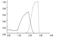
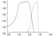
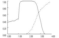
Figure 5 clearly
demonstrates the interaction effects. In all three games, fixation reduces cooperation
at low aspiration levels and increases cooperation at high aspiration levels.
Fixation also shifts the optimal balance point for aspirations to a level close
to the R payoff of the game, or A = 3 in PD and Chicken and A = 4 in Stag Hunt. In
addition, the figure reveals that the interaction between fixation and low
aspirations does not depend on whether aspirations are below or above the
maximin payoff. As long as aspirations levels fall below A = 2, moderate fixation (f = 0.5) suppresses random walk into mutual cooperation.
However, the mechanisms
differ, depending on whether aspirations are above or below maximin. Below maximin, the predominant
self-reinforcing equilibria are deficient outcomes, mutual defection in the
Prisoner’s Dilemma and Stag Hunt and unilateral cooperation in Chicken. These
equilibria prevail at low aspiration levels because their coordination
complexity is considerably lower than that of mutual cooperation. Accordingly,
fixation reduces cooperation in this region because it increases the odds that
learning dynamics converge on the SRE that is easiest to coordinate, at the
expense of mutual cooperation. With aspirations levels above maximin, fixation
no longer induces convergence on a deficient SRE, but it inhibits convergence
on the unique SRE of mutual cooperation.
To sum up, the GRL
model shows that stochastic collusion is a fundamental solution concept for all
social dilemmas. However, we also find that the viability of stochastic collusion
depends decisively on the assumptions about fixation. With high aspirations,
fixation makes stochastic collusion more likely, while with low aspirations, it
makes cooperation more difficult.
3.3 Self-correcting equilibrium and fixation
We
now use low learning rates to study the effect of fixation on the stability of
the socially deficient SCE. The coordination complexity of random walk
increases exponentially as the learning rate decreases. In our baseline
condition with A = 2 and f = 0, but a low learning rate of l = 0.05, stochastic collusion
is effectively precluded in all three social dilemma games, even after 1000
iterations and with moderate aspiration levels. We confirmed this by measuring
mean cooperation in the 1000th iteration over 1000 replications. For
all three types of social dilemma, the mean was not statistically different
from the SCE derived analytically from the payoffs (p = 0.366 for PD and p
= 0.5 for Chicken and Stag Hunt).
We want to know if
fixation makes it easier to escape and whether this depends on the level of
aspirations. To find out, we crossed fixation (f = 0 and f = 0.5)
with aspirations just above maximin (A = 1.05)
and just below minimax (A = 2.95), just as we did in
the previous study of stochastic collusion with high learning rates.
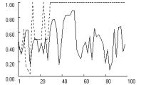
When aspirations are
low, the predominance of reward over punishment should cause the effective
learning rate to decline as players fixate on repeated reward. With the
baseline learning rate already near zero, fixation should have little effect,
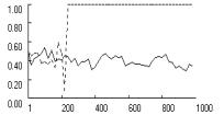
and this is confirmed in Figure 6, based on 1000 iterations in each of the
three games. Reduction in the effective learning rate merely smooths out fluctuations
in players’ probability of cooperation, pc
, around an equilibrium level of about pc
= 0.13 in the Prisoner’s Dilemma, and pc
= 0.5 in Chicken and Stag Hunt, respectively. Reliability tests showed a slight
negative effect of fixation on the equilibrium rate of cooperation. Based on
1000 replications, we found that in the PD and Chicken, the rate of stochastic
collusion within 1000 iterations was zero, with or without fixation. In Stag
Hunt, stochastic collusion remained possible without fixation (with a rate of
0.21), but this rate dropped to zero with f = 0.5.
In short, without fixation, the low learning rate of l = 0.05 allows players to escape the SCE only in Stag
Hunt. Fixation suppresses even this possibility.
|
|
|
|
|
Prisoner’s Dilemma (T>R>A>P>S) |
Chicken (T>R>A>S>P) |
Stag Hunt (R>T>A>P>S) |
|
Figure
6. Effects of fixation (dotted line) on SCE with low learning
rates and low aspirations in three social dilemma games (p = [4,3,1,0], l = 0.05, A = 1.05,
f = [0, 0.5], qc,1 = qd,1 = 1). |
||
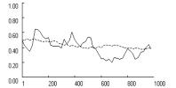
With high aspirations - and a predominance
of punishment over reward - fixation should have the opposite effect,
causing the effective learning rate to increase. This in turn should make
stochastic collusion a more viable solution. To test this possibility, we increased
the aspiration level to A = 2.95.
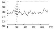
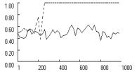
Figure 7 confirms the
expected cooperative effect of fixation when aspirations are high. The increase
in the effective learning rate helps players escape the SCE within about 250
iterations in all three games. Reliability tests show a very powerful effect of
fixation. With f = 0, the
rate of stochastic collusion within 1000 iterations is zero in all three games.
With moderate fixation (f = 0.5),
stochastic collusion within 1000 iterations becomes virtually certain in all
three games.
|
|
|
|
|
Prisoner’s Dilemma (T>R>A>P>S) |
Chicken (T>R>A>S>P) |
Stag Hunt (R>T>A>P>S) |
|
Figure 7. Effects of fixation (dotted line) on SCE
with low learning rates and high aspirations, in three social dilemma games (p = [4,3,1,0], l = 0.05,
A = 2.95, f = [0, 0.5], qc,1 = qd,1 = 1). |
||
As an additional test,
we varied the aspiration level A from
0 to 4 in steps of 0.1, exactly as in Figure 5, only this time, with a low
baseline learning rate. The results confirm that fixation largely cancels out
the effects of a low learning rate. Without fixation (f = 0), stochastic collusion is effectively precluded by
a low learning rate, regardless of aspiration levels. With fixation, the rate
of stochastic collusion over 1000 iterations was virtually identical to that
observed in Figure 5 with a high baseline learning rate.
To sum up, without
fixation, low baseline learning rates make it very difficult for
backward-looking actors to escape the social trap, regardless of aspiration
levels. However, if aspirations are high, fixation increases the effective
learning rate to the point that escape becomes as likely as it would be with a
moderate baseline learning rate. If aspirations are low, fixation reduces the effective
learning rate, but since the rate is already too low to attain stochastic
collusion, there is little change in the outcome.
4. Discussion and Conclusion
Concerns
about the Nash equilibrium as solution concept for the analysis of
interdependent behavior have led cognitive game theorists to explore
learning-theoretic alternatives. Two prominent examples are the BM stochastic
learning model and the RE payoff-matching model. Both models identify two new
solution concepts for the problem of cooperation in social dilemmas, a socially
deficient SCE (or social trap) and a self-reinforcing equilibrium that is
usually (but not always) socially efficient. The models also identify the
mechanism by which players can escape the social trap - stochastic collusion, based on a random walk in
which both players wander far enough out of the SCE that they escape its
“gravitational” pull. Random walk, in turn, implies that a principle obstacle
to escape is the coordination complexity of stochastic collusion.
It is here - the effect of
learning rates on stochastic collustion - that the two learning models diverge. The
divergence might easily go unnoticed, given the theoretical isomorphism of two
learning theoretic models based the same three fundamental behavioral
principles – experiential induction (vs. logical deduction), reward and
punishment (vs. utility), and melioration (vs. optimization). Yet each model
implements these principles in different ways, and with different results. In
order to identify the differences, we aligned and integrated the two models as
special cases of a GRL model. The integration and alignment uncovered a key
hidden assumption, the “Power Law of Learning.” This is the curious but
plausible tendency for learning to diminish with success and intensify with
failure, which we call “fixation.” Fixation, in turn, impacts the effective
learning rate, and through that, the probability of stochastic collusion.
We used computer
simulation to explore the effects of fixation on stochastic collusion in three
social dilemma games. The analysis shows how the integration of alternative
models can uncover underlying principles and lead to a more general theory.
Computational experiments confirmed that stochastic collusion generalizes
beyond the particular BM specification. However, we also found that stochastic
collusion depends decisively on the interplay of fixation with aspiration
levels and the baseline learning rate. The GRL Model shows that, in the absence
of fixation, the viability of stochastic collusion is compromised by low
baseline learning rates and both low and high aspirations. With low
aspirations, actors learn to accept socially deficient outcomes as “good
enough.” We found that fixation exacerbates this problem. When rewards dominate
punishments, fixation reduces the effective learning rate, thereby increasing
the coordination complexity of stochastic collusion via random walk.
With high aspirations,
actors may not feel sufficiently rewarded by mutual cooperation to avoid the
temptation to defect. Simulations show that fixation removes this obstacle for
stochastic collusion, so long as aspirations do not exceed the payoff for
mutual cooperation. High aspirations cause punishments to dominate rewards.
Fixation then increases responsiveness to stimuli, facilitating random walk
into the basin of attraction of mutual cooperation.
Our exploration of
dynamic solutions to social dilemmas is necessarily incomplete. Alignment and
integration of the BM and RE models identified fixation as the decisive
difference, and we therefore focused on its interaction with aspiration levels,
to the exclusion of other factors (such as Schelling points and network
structures) that also affect the viability of stochastic collusion. We have
also limited the analysis to symmetrical two-person simultaneous social dilemma
games within a narrow range of possible payoffs. Previous work (Macy 1989,
1991) suggests that the coordination complexity of stochastic collusion in
Prisoner’s Dilemma increases with the number of players and with payoff
asymmetry. We leave these complications to future research.
The identification of
fixation as a highly consequential hidden assumption also points to the need to
test its effects in behavioral experiments, including its interaction with
aspiration levels. Both the BM and the RE models have previously been tested experimentally, but these
tests did not address conditions that allow discrimination between the models
(Macy 1995, Erev and Roth 1998). Our research identifies these conditions.
Erev, Roth and others (Roth and Erev 1995; Erev and Roth 1998; Erev et al.
1999) estimated parameters for their payoff-matching model from experimental
data. However, empirical results can not be fully understood if key assumptions
are hidden in the particular specification of the learning algorithm. Their
learning algorithm “hardwires” fixation into the model without an explicit
parameter to estimate the level of fixation in observed behavior. Theoretical
integration of the two models can inform experimental research that tests the
existence of fixation and its effects on cooperation in social dilemmas,
including predicted interactions with aspiration levels.[7]
Given the theoretical
and empirical limitations of this study, we suggest that its primary contribution
may be methodological rather than substantive. By aligning and integrating the
Bush-Mosteller stochastic learning model with the Roth-Erev payoff-matching
model, we identified a hidden assumption - the Power Law of Learning - that has been
previously unnoticed, despite the prominent position of both models in the
game-theoretic literature. Yet the assumption turns out to be highly
consequential. This demonstrates the importance of “docking” (Axtell et al.
1996) in theoretical research based on computational models, a practice that
remains all too rare. We hope this study will motivate greater appreciation not
only of the emerging field of cognitive game theory but also of the importance
of docking in the emerging field of agent-based computational modeling.
References
Axelrod, R. 1984. The Evolution of Cooperation. New York: Basic Books.
Axelrod and Cohen. 2000. Harnessing Complexity. Organizational
Implications of a Scientific Frontier. New York: Basic Books.
Axtell, R., R. Axelrod, J. Epstein and M. Cohen.
1996. “Aligning Simulation Models: A Case Study and Results.” Computational and Mathematical Organization
Theory 1:123-141.
Blackburn, J.M. 1936. “Acquisition of Skill: An
Analysis of Learning Curves.” IHRB Report
73. (Reference taken from Erev and Roth 1998).
Catania, A. C. 1992. Learning (3rd ed.). Englewood Cliffs, NJ: Prentice Hall.
Cohen, M.D., R. L. Riolo and R. Axelrod. 2001.
“The Role of Social Structure in the Maintenance of Cooperative Regimes.” Rationality and Society 13(1):5-32.
Dawes, R.M 1980. “Social Dilemmas.” Annual Review of Psychology 31:169-193.
Dawes, R.M., R.H. Thaler. 1988. “Anomalies: Cooperation.”
Journal of Economic Perspectives
2:187-197.
Erev, I., Y. Bereby-Meyer and A.E. Roth. 1999.
“The Effect of Adding a Constant to all Payoffs: Experimental Investigation and
Implications for Reinforcement Learning Models.” Journal of Economic Behavior and Organization 39: 111-128.
Erev, I. and A.E. Roth. 1998. “Predicting how
People play Games: Reinforcement Learning in Experimental Games with Unique,
Mixed Strategy Equilibria.” American
Economic Review 88(4):848-879.
Fischer, I. , R. Suleiman. 1997. “Election
Frequency and the Emergence of Cooperation in a Simulated Intergroup Conflict.”
Journal of Conflict Resolution 41
(4):483-508.
Flache, A. 1996. The Double Edge of Networks. An Analysis of the Effect of Informal
Networks on Cooperation in Social Dilemmas. Amsterdam: Thesis Publishers.
Fudenberg, D. and D. Levine. 1998. The Theory of Learning in Games. Boston:
MIT Press.
Homans, G.C.
1974. Social Behavior. Its Elementary
Forms. New York: Harcourt Brace Jovanovich.
Herrnstein, R.J. and P. Drazin 1991.
“Meliorization: A Theory of Distributed Choice.” Journal of Economic Perspectives, Vol. 5, No. 3, pp. 137-156.
James, W. 1981. Principles of Psychology. Cambridge: Harvard University Press.
Kanazawa, S. 2000. “A New Solution to the
Collective Action Problem: The Paradox of Voter Turnout.” American Sociological Review.
Liebrand, W.B.G. 1983. “A Classification of
Social Dilemma Games.” Simulation &
Games 14:123-138.
Macy, M.W. 1989. “Walking out of Social Traps: A
Stochastic Learning Model for the Prisoner's Dilemma.” Rationality and Society 2:197-219.
Macy, M.W. 1990. “Learning Theory and the Logic
of Critical Mass.” American Sociological
Review 55:809-826.
Macy, M.W. 1991. “Learning to Cooperate:
Stochastic and Tacit Collusion in Social Exchange.” American Journal of Sociology 97:808-843.
Macy, M.W. 1995. “PAVLOV and the Evolution of
Cooperation: An Experimental Test”.
Social Psychology Quarterly 58(2):74-87.
Macy, M.W., A. Flache. 2002. “Learning Dynamics
in Social Dilemmas.” Proceedings of the National Academy of Sciences
U.S.A. 99:7229-7236.
March, J.G. and H. A. Simon. 1958. Organizations. New York: Wiley.
Peyton Young, H. 1998. Individual Strategy and Social Structure. An Evolutionary Theory of
Institutions. Princeton, N.J.: Princeton University Press.
Rapoport, A. and A.M. Chammah. 1965. Prisoner's Dilemma: A Study in Conflict and Cooperation. Ann Arbor: Michigan University Press.
Raub, W. 1988. “Problematic Social Situations
and the Large Number Dilemma.” Journal of
Mathematical Sociology 13:311-357.
Roth A.E. and I. Erev. 1995. “Learning in
Extensive-Form Games: Experimental Data and Simple Dynamic Models in
Intermediate Term.” Games and Economic
Behavior. Special Issue: Nobel Symposium 8, 164-212.
Rummelhart, David E. and James L. McLelland.
1988. Parallel Distributed Processing:
Explorations in the Microstructure of Cognition. Cambridge, MA: MIT Press.
Thorndike, E.L. 1898. Animal Intelligence. An Experimental Study of the Associative Processes
in Animals. Psychological Monographs 2.8.. (reprinted 1999 by Transaction;
page number may be different in new edition).
Weibull, J.W. 1998. “Evolution, Rationality and
Equilibrium in Games.” European Economic
Review 42:641-649.
Appendix
We
prove that without fixation (f = 0)
our Generalized Reinforcement Learning Model is equivalent to the BM stochastic
learning model in equations [1] and [2]. By extension, we also obtain the
original learning mechanism of Roth and Erev as a special case of a BM
stochastic learning model with a dynamic learning rate.
To derive the equation
for the effective change in choice probabilities, we use the probabilistic
choice rule [4] with the propensities that result after the reinforcement
learning rule [5] has been applied in round t.
Without loss of generality, let a be
the action carried out in t. Equation
[A.1] yields the probability for action a
in round t+1, pa,t+1 , as a function of the reinforcement and the
propensities in t:
![]() [A.1]
[A.1]
Suppose, a was rewarded, i.e. sa,t ³ 0. Substitution of the response function r in [A.1] by rG with f = 0
yields, after some rearrangement, equation [A.2]:
![]() . [A.2]
. [A.2]
In equation [A.2], we
substitute the terms corresponding to the right hand side of the probabilistic
choice rule [4] by the choice probabilities in round t, pa,t and pb,t
= 1 - pa,t,
respectively. Equation [A.2] then yields the new choice probability as a
function of the old choice probability and the reinforcement. Equation [A.3]
shows the rearrangement, where (a,b) Î {C,D} and a¹b:
![]() [A.3]
[A.3]
The
right hand side of [A.3] is equivalent to the BM updating of probabilities
following “upward” reinforcement (or increase of propensity), defined in [2].
The BM equations for
punishments of a are obtained in the
same manner. Let sa,t
< 0. Then, substitution of the response function rG with f = 0
in equation [A.1] yields after some rearrangement the new probability for
action a, given in [A.4]:
![]() [A.4]
[A.4]
Again, substitution of
the terms for pa,t and pb,t = 1 - pa,t according to the
probabilistic choice rule yields the new probability as the function of the
preceding probability and the punishment that is specified by Equation [A.5].
![]() [A.5]
[A.5]
The
rightmost expression in equation [A.5] is identical with the BM stochastic learning
rule for “downward” reinforcement (or reduction of propensity) defined in [2].
We now show that the
original Roth-Erev learning mechanism with response function rRE can also be obtained as a
special case of a BM learning algorithm with a dynamic learning rate. Consider
the case where action a was taken in t and rewarded (sa ³ 0). In the BM algorithm, the new probability pa,t+1 for action a is given by equation [2] above. To
obtain the corresponding RE learning rule, we express the learning rate in the
BM equation as a function of the present propensities and the most recent
payoff. More precisely, the BM equation [2] expands to the RE equations [4] and
[5] if the learning rate l is
replaced as follows:
![]() . [A.6]
. [A.6]
Equation
[A.6] shows that for rewards, the RE model is identical to the BM, with a
learning rate that declines with the sum of the net payoffs for both actions in
the past.
To obtain the BM
equation for punishment, the corresponding learning rate function for
punishment of action a is
![]() [A.7]
[A.7]
Equation [A.7] modifies
the learning rate as in [A.6], but it also ensures that the learning rate is exponentially amplified as the propensity
for the action taken approaches zero. This forces the behavior of the original
RE model onto the BM equations. Now the
corresponding action propensity drops discontinuously down to its lower bound,
a behavior that the BM model with a constant learning rate l avoids with the dampening term l sa pa., as pa moves towards zero. Conversely, [A.7] decreases the
learning rate as the propensity for the alternative action b approaches zero. The latter effect of [A.7] obtains when the
probability for action a is close to
1. In that case, the BM model with a constant learning rate l implies a rapid decline of the
propensity of a after punishment,
unlike the RE model. Equation [A.7] again forces RE behavior onto the BM equations,
as the declining learning rate modifiesthe strong effect of punishment in this
condition.