Comparing individual-based model of behaviour diffusion with its mean field aggregated approximation

Margaret Edwards, Sylvie Huet, François Goreaud, Guillaume Deffuant

Margaret.Edwards@CLERMONT.cemagref.fr

Laboratoire d’Ingénierie des Systèmes Complexes
Cemagref
24, av. des Landais
63 000 Aubière

Abstract

We compare the individual-based “threshold model” of innovation diffusion (Valente 95), in the version which has been studied by P. Young, and an aggregate deterministic model we constructed from it. The classical threshold model supposes that an individual adopts a behaviour according to a trade-off between a social pressure (the number of his neighbours adopting the behaviour) and a personal interest or resistance to change (the threshold). The aggregate model makes approximations in order to estimate the evolution of groups of individuals with the same number of neighbours of similar behaviour. We compare both models in different points of the parameter space. We find that the aggregate model gives a good approximation of the individual when the individual based model is very stochastic. When the individual based model is less stochastic, the behaviour of the aggregate approximation differs ; it is attracted by local equilibrium points which are not the most probable state (dominant equilibrium point) of the individual-based model. Our theoretical interpretation of this difference is based on a study of the attractors of both dynamics.

1 Introduction

Individual-based models are more and more commonly used in ecological modelling (Grimm 1999), or to model social and economical processes (Gilbert and Troitzch 1999). An explanation of this growing interest is that individual based models can incorporate very detailed and refined representations of the individuals and their behaviour. It is expected that this growing level of details brings more realism in the model, which becomes a more faithful representation of the reality. However, such detailed descriptions lead to heavier computational models which are sometimes very difficult to understand.

Individual based models can be opposed to models ruling directly the dynamics of aggregated variables describing a population. Aggregate models have the advantage of shorter computation times and their mathematical form provides theoretical insights on their possible behaviour, before any simulations are performed, or useful elements to explain the results. Moreover, administrators and managers are often in general interested by aggregate variables, such as the number of individuals, their distribution of ages, the global biomass.

It is therefore important to understand in which conditions the development of an individual based model will actually bring some additional insight to the studied phenomenon. For instance, if the additional complexity of the individual based model does not bring any difference in the global behaviour, then aggregate models are certainly more appropriate.

Recent studies have sought to compare individual-based to aggregate models. DeAngelis and Rose (1992) study the influence of transforming continuous variables into discrete distributions in models of ecological dynamics ; Picard and Franc (2001) show that space-dependant individual based models and aggregated models (regarding either spatial influence or description of the population) of forest dynamics lead to different results. Fahse et al. (1998) and Duboz et al. (2002) use individual-based models to extract parameters for population-level dynamics.

We study this question for a particularly well studied innovation diffusion model, sometimes called the threshold model (Valente 1995, Grannovetter 1978). Its principle is that the behaviour of an agent is influenced by a the behaviour of its neighbours (in general with a tendency to imitation), and by an intrinsic interest for one or the other behaviour. It can be interpreted as a decision based on a utility function which performs a trade-off between a social pressure and an individual interest. This model is by nature individual based because it relies on the interactions of each individual with its neighbours (or associates in a social network). Different variants of this model are well studied and a theory of its behaviour is also available (Young 1998).

We propose an aggregate version of this model which is based on a mean field approach. We consider aggregated variables which are the proportion of the population adopting each behaviour, and consider the master equation ruling the flow from each state to the other. Such an approach is common in the socio-dynamics (Weidlich, Elbing, Faure et al.). In order to simplify this computation, we suppose that the social network is of the same size for all the agents (which is not the case in the individual based model).

We show that the results of the individual and aggregate models can be very close or very different, depending on the chosen parameters. For some parameters, the aggregate model is trapped in local minima, whereas the individual based model, because of its stochasticity always gets out from these local minima.

We first present the individual and aggregated models. Then we propose some examples of simulations where their behaviour are similar, and others where they are significantly different. Finally, we propose an theoretical explanation of these results.

2 Aggregating an individual based model of innovation diffusion

2.1 The individual based model of innovation diffusion

The threshold model is initially inspired from the sociology of innovation diffusion. Its principle is that the decision of an agent to change its behaviour relies on a trade-off between a social pressure (considering the behaviour of its neighbours), and an intrinsic, personal interest.

We consider here the stochastic version of the model. We recall hereafter the main features of this model. More details can be found in (Young, P. 1999).

We consider N agents, having the choice between two behaviours : A and B. N is constant over time. Each agent i has a social network V(i). In our experiments the social network is randomly drawn : we define a priori a number of links for the whole population, and pick the links at random. The social network is therefore characterised by an average number of links v for an individual.

The choice to adopt either the A or the B behaviour ensues from utility computation. The utility U_i(A) and U_i(B) of agent i to choose A or B is expressed as :

where V(i,A) and V(i,B) are the number of neighbours of agent i respectively of behaviour A or B and the g_XY are parameters of the model.

In order to take into account individual variability and uncertainty in the decision, Young introduces a stochastic response: the probability for an individual i of adopting A or B is :

For b=0, the function is purely random ; for b ®¥ , this function becomes quasi deterministic.

2.2 Aggregating and mean field approximation

We build the aggregate model within the socio-dynamics (Weidlich, Elbing, Faure) approach which inspired from physics. The principle is to consider the evolution of the probability distribution in the states of the model, ruled by the “master equation”. In the case of the mean field approximation, we consider only the evolution of the mean of this probability distribution. Moreover, we suppose that all the agents have the same number of neighbours v.

We define the state of the system by a vector of the number of agents with behaviour A having 0, 1…v neighbours with behaviour A, and similarly for agents of behaviour B. We call the number of agents with behaviour A and k neighbours of behaviour A. Similarly, we call the number of agents with behaviour B and k neighbours of behaviour A. The state s(t) of the model is therefore a vector of dimension 2v+2 :

Suppose that there are agents of behaviour A in the population (and agents with behaviour B). We approximate as proportional to the probability to pick k agents with behaviour A among v picked at random in the population. This probability is given by the binomial formula :

From which we derive :

Similarly, we have :

Moreover, for each agent in , the probability to choose B is given by :

Similarly, for any agent in , the probability to choose A is given by :

We can approximate the number of agents which will change their behaviour into B :

This allows us to evaluate the evolution of the number of agents A in the population :

Which finally leads to :

For the simulations we round up these values to the closest integer. This gives us the new value of , and we can compute the value of s(t+1), and iterate again.

3 Experimental comparisons

We have run comparative simulations for two series of parameters.

In both cases we have a=3, b=2, c=d=0.

In the first case, b=0.1 and in the second b=0.6.

We expected that the aggregate model would approximate well the mean results from the individual-based model. But we observe that in the first case the results are very similar, whereas in the second appear differences which are then interpreted in section 4.

3.1 With b = 0.15 the models have similar behaviours

For A =3, b =2 and b = 0.15 the aggregate model approximates the mean dynamics of the individual-based one.

In figure 1 appear the proportion of A over time for the aggregate model and for the individual-based model, for an initial proportion of A behaviour is here 0. The aggregate model is deterministic and provides a single value. The individual-based model is stochastic. We have shown the mean value for 150 simulations ; the minimum and maximum moreover give an idea of the range of values possibly computed by the individual-based model for this set of parameters.

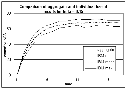
Figure 1. Comparison of the results of the aggregate with the individual-based model for b = 0.15, for which out of 150 simulations are represented the minimum, the maximum and the mean values. The trends are very similar.

From an initial proportion of 0% A behaviours in the population, both models tend towards a value around 68%, which seems to be an equilibrium. At every time step, the results of the aggregate model are very close to the mean calculated from the individual-based model’s simulations.

Here the hypothesis we made to construct the aggregate model seem to be justified, since the aggregate model provides a good estimation of the evolution of the individual-based model.

3.2 With b = 0.6 the models exhibit different behaviours

We performed a second series of simulations with similar parameters for the payoff matrix (a=3, b=2, c=d=0) but with b=0.6., and different initial values of A behaviours in the population. Here we observe differences between the two models. Before explaining these differences and showing how the aggregate model gives us useful elements to understand the individual-based one (in section 4.), we describe the differences we observed.

The most probable states computed by the two models are not always the same : whereas P. Young showed in his paper that the most likely state on long run is 100% of individuals in A for any initial proportion of A behaviours (which appears in the simulations), on the contrary the final value of deterministic aggregate model depends on this initial proportion.

Hereafter we present two sets of simulations for initial proportions of A behaviours in the population of 15% and 23%.

3.2.1 Comparison for an initial proportion of A behaviours of 23%

In figure 2 we show the results of the individual-based and the aggregate models for an initial proportion of A behaviours of 23%. For the individual-based model we have represented the mean value at each time step, calculated over 150 simulations.

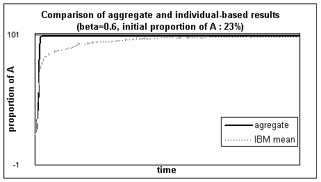
Figure 2. Comparison of the results of the aggregate with the individual-based model, for which we have represented the mean over 150 simulations, for b = 0.60 and initially 23% A behaviours.

The results of the two models show the same most probable state ; it is of 100% A behaviours for the individual-based model, as P. Young showed it in his paper, and as the mean results of the simulations seem to show it here ; the deterministic aggregate model reaches this state, where it stays ; since its evolution depends only on the proportion of A behaviours in the population, this state is the final state, and is the most probable over time.

But the aggregate model converges faster than the mean value of the individual-based model ; it doesn’t approximate the mean values of the individual-based model over the time as closely as for the previous set of parameters.

Finally, both models tend towards 100% of A behaviours, but in slightly different ways.

3.2.2 Comparison for an initial proportion of A behaviours of 15%

We have performed similar comparison for an initial proportion of A behaviours of 15%.

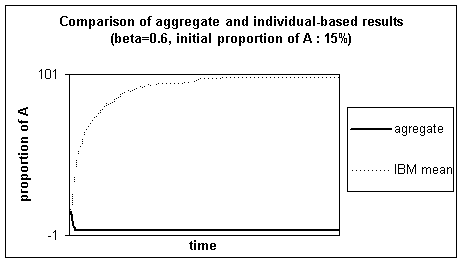
Figure 3. Comparison of the results of the aggregate with the individual-based model, for which the mean out of 150 simulations is represented, for b = 0.60 and initially 15% A behaviours.

The behaviours of the two models are very different.

The individual-based model tends towards 100% A behaviours, which is it’s most probable state (as P. Young showed).

On the contrary, the aggregate model leaves quickly the confidence interval for the results of the individual-based model ; it’s final state is 0% A behaviours.

These results seem to indicate the existence of more than one point of equilibrium, met by the aggregate model because of it’s determinism. In the next section we will detail elements to characterise the aggregate model’s dynamics and confirm this hypothesis, and see how these elements might be useful to characterise the individual-based model’s dynamics.

4 Theoretical explanation of the experiments

4.1 Stochastic attractor of the individual based dynamics (P. Young)

P. Young defines the following potential which determines here the states of equilibrium.

Where x is the vector of choices of the individuals, and A(x) (respectively B(x)) represents the number of links between two individuals with A (respectively B) behaviours. We see that all-A or all-B are locally stable states, since the change in opinion of a single individual can only lead to a decrease of this potential.

Thereafter P. Young characterises the almost sure frequency m^b(x) with which a state x is visited over the long run.

Therefore the most likely state x is the one that maximises the potential function r(x). However, note that all states have a strictly positive probability to appear (even though it can be very small).

4.2 Classical equilibrium points of the aggregate dynamics

In order to get a closer idea of the evolution of the aggregate model, we seek to define similarly a potential for characterising equilibrium states and dynamics of this model.

We deduce from the evaluation of flows between behaviours used for constructing the aggregate model, the increase dA in A behaviours in the population between t and t+d for a given initial proportion of A.

In this way we estimate an approximate derivative of the evolution of proportion of A in the population over. A unit time step is defined as the time necessary for the re-evaluation of behaviours for the whole population, following the rules proposed by Young.

The following figure represents for b=0,6 an approximation of the derivative and the potential associated, whose minima describe the stable states of equilibrium (and the maxima, the unstable ones).

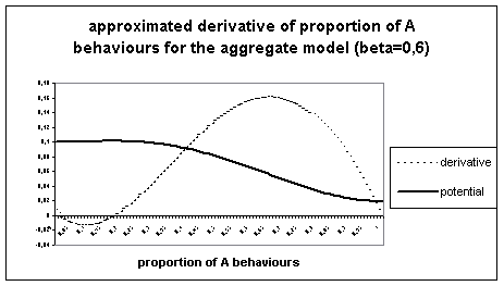
Figure 4. Approximated derivative of the aggregate calculation of proportion of A for b=0,6.

We notice this derivative meets zero in three points, corresponding to local extrema of the potential function. The two extreme points correspond (as expected) to the final states found for the aggregate model, confirming the trends observed in the aggregate model simulations. Moreover we see that these points are stable, and that there exists an unstable intermediate point of equilibrium, which delimits the attraction basins for the stable equilibrium points.

For values smaller than the intermediate equilibrium point, derivative is negative, causing the proportion of A behaviours to decrease ; this explains the quick trend towards 0 observed in the aggregate case.

For values greater than this point, on the contrary, derivative is positive, provoking increase of the A behaviours in the population.

For this combination of parameters where more than one equilibrium point exist, the initial value is decisive for the final state of the aggregate model, whereas indifferent for the individual-based one. Since this model is deterministic, once passed this threshold for change, it follows the trend defined by the derivative. Therefore it reaches equilibrium points which are stable for him. On the contrary the individual-based model always reaches the dominant equilibrium point by it’s stochasticity, which acts like simulated annealing.

Conversely let’s consider a similar diagram for b=0.15, to confirm this derivative leads to equilibrium points.

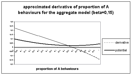
Figure 5. Approximated derivative of the aggregate calculation of proportion of A, for b=0.15.

We see here there is a unique point of equilibrium met by both models.

This explanation of divergence between the two models seems satisfactory : the aggregate model because of it’s determinism, meets equilibrium points which the individual-based model avoids with it’s stochasticity (following the principle of simulated annealing), so that it’s most probable state depends only on the value of the parameters (as P. Young predicts).

5 Discussion : elements possibly useful for characterising the individual-based model’s dynamics ?

Since the main difference between the two models seems to be due to their deterministic versus stochastic behaviour, one can wonder whether the formalism proposed by the aggregate model can provide interesting indications for the individual-based model’s dynamics, by and outside these observed differences : first by the influence of b on the mean state for finite number of time steps ; secondly on the evolution over time of the individual-based model (and the laps of time necessary to get to the most probable state).

5.1 Influence of b on the mean final state

We observe and compare the final states : predicted by the aggregate model and observed from the individual-based simulations, for small values of b. In this case the behaviour of the models is close to pure randomness.

We have represented the stable and unstable points of equilibrium computed for the aggregate model from its derivative and potential ; and the “mean state” of the individual-based model (over 5000 time steps) ; to evaluate it, we consider the evolution of the mean computed over the simulations, for one time step; we then mean over time this one-time-step mean, from the first point where it doesn’t increase and varies only little (so seems to reach stability), until the end of the simulations (this is always over half of the time steps). This mean state theoretically depends on the weighting (defined by b) on the equilibrium states of the individual-based model.

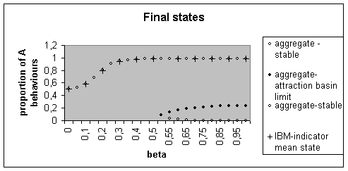
Figure 6. Different equilibrium states for the aggregate model and mean final states for the individual-based model, for different values of b.

The aggregate model has only one (for b<0.52), then two stable equilibria. The existence of an unstable intermediate equilibrium point defines the limits of the attraction basins for the two stable equilibrium points. We see that the basin around 0 is smaller than the one around 1, which seems to echo the dominance of 1 (all-A) in the individual-based model.

For the individual-based model, for very small values of b, the weighting of the different equilibrium points is very close, thereby favouring an intermediate state. The more b increases, the more the dominance of the all-A state appears, by nearing the mean state to 100% A behaviours. (For b higher than 1 (up to 50), the mean state for the individual-based model, and for the aggregate model the equilibrium points and the limit of the attraction basins do not vary much.)

The equilibrium points of the aggregate model seem to foresee well this mean-state indicator for the individual-base model.

5.2 Dynamic evolution

Do the existence of a second equilibrium point, and the limit of its attraction basin described by the aggregate model find an echo in the individual-based model ?

In order to find out, we consider the dynamics of the individual-based model over time, for the studied set of parameters where there appeared to be more than one equilibrium points for the aggregate model (b=0,6). If the individual-based simulations are sensitive to an attraction basin around 0 (for the proportion of A behaviours in the population), the progress should be slower when starting there.

To check this we observe the mean time to get to 95% A behaviours (for 150 simulations), from different initial proportions.

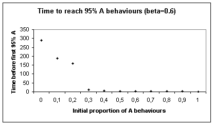
Figure 7. Time to reach 95% A behaviours for the individual-based model, depending on the initial proportion of A behaviours

The time to reach 95% A behaviour does not depend linearly on the initial proportion of A behaviour.

If the initial proportion is higher than a value close to the limit of the 0-A attraction basin in the aggregate case (between 0.2 and 0.3), the progression is very fast. This corresponds to a positive derivative in the aggregate model (this is : a tendency to increase the proportion of A behaviours). Under this initial value, on the contrary, time increases suddenly very fast with the distance, as though the trend towards 1-A was delayed by contrary trends and/or more subject to the uncertainty induced by the stochasticity. This corresponds for the aggregate model to a negative derivative of small absolute value.

So the behaviour showed by the simulations of the individual-based model seems to echo to the existence of a 0-A attraction basin for the aggregate model.

Therefore it seems that the aggregate model gives us aggregate indicators which seem pertinent to describe the evolution of the individual-based model.

6 Conclusion and perspectives

From the individual-based decision model studied par P. Young, we have constructed an aggregate model which describes at population level the evolution of the proportions of the behaviours. Its results show that this model approximates the mean value of the results provided by the individual-based model, in some cases.

We have identified, interpreted and characterised a cause of divergence between the two models, by constructing an approximate derivative from the aggregate model. In the case where the parameters define more than one equilibrium points, the aggregate model is sensitive to initial conditions, which can lead it to local equilibrium states. The individual-based model avoids these by its stochasticity, which has the effect of simulated annealing.

If the aggregate model because of its determinism doesn’t approach the behaviour of the individual-based model in all cases, it provides nevertheless interesting theoretical elements to understand and characterise the individual-based model’s behaviour at an aggregate level.

7 References

Axelrod, R. (1995) “The convergence and stability of cultures : local convergence and global polarization”. Ann Arbor, Institute of Public Policies Study, University of Michigan : 34

Blume, L (1993) “The statistical mechanics of strategic interaction”. Games and economic behaviour 4:387-424

Blume, L (1995) “The statistical mechanics of best-response strategy revision”. Games and economic behaviour 11:111-145

DeAngelis, D.L. ; Gross, L.J. Editors (1992) : “Individual-based models and approaches in ecology”, Chapmann & Hall

Duboz, R. ; Ramat, E. ; Preux, P. (2002) “Scale transfer modelling : using emergent computation for coupling an ordinary differential equation system with a reactive agent model”

Ellison, G (1993) “Learning, Social interaction, and coordination”. Econometrica 61:1047-71

Epstein, J. ; Axtell, R. (1996) “Growing artificial Societies : Social science from the bottom up”. Cambridge Massachussetts, MIT Press

Fahse, L ; Wissel, C. ; Grimm, V (1998) “Reconciling Classical and Individual-Based Approaches in Theoretical Population Ecology : A Protocol for Extracting Population Parameters from Individual-Based Models”

Faure, T. ; Deffuant, G ; Weisbuch, G (2002) “Dynamics of influence on continuous incertain opinions : Evolution of the opinion porbability distribution”, submitted

Gilbert, N. ; Troitzsch (1999) “Simulation for the social scientists” Open university press.

Granovetter, M. (1978) “Threshold models of collective behaviour”. American journal of sociology 83:1360-1380

Grimm, V., 1999. “Ten years of individual-based modelling in ecology: what we have learned and what could we learn in the future ?”, Ecological Modelling, 115, p.129-148, 1999.

Maienhofer, T. F. (2001) « Finding optimal targets for change agents : a computer simulation of innovation diffusion”.

Morris, S. (1997) “Contagion”. Working paper, department of economics, university of Pennsylvania.

Picard, N. ; Franc, A. : (2001) “Aggregation of an individual-based space-dependant model of forest dynamics into distribution-based and space-independant models”, Ecological Modelling.

Valente, T.W. (1995) “Network models of the diffusion of innovations”. Cresskill, New Jersey, Hampton Press, Inc.

Weidlich, W (2000) “SocioDynamics, A Systematic Approach to Mathematical Modelling”, Harwood academic publishers

Young, P. (1998) “Individual Strategy and social structure”, Princeton University Press

Young, P. (1999) “Diffusion in Social Networks”, Working Paper No 2., Brookings Institution

Improving agri-environmental policies : a simulation approach to the cognitive properties of farmers and institutions, final report, version 2 (October 2001), FAIR3 CT 2092