Individual-based model to enrich an aggregate
model
Raphaël Duboz* *, Frédéric Amblard**, Eric Ramat*, Guillaume Deffuant**, Philippe Preux*
|
*Laboratoire d'Informatique du Littoral (LIL) Maison de la Recherche Blaise Pascal |
**Laboratoire d'Ingénierie pour les Systèmes Complexes (LISC) Cemagref 24, avenue des Landais BP 50085 63172 Aubière Cedex France |
*
Email: duboz@lil.univ-littoral.fr
tel:
+33 321 465 679
Abstract:
We propose to use individual-based models as virtual laboratories to identify
parameters of aggregate models. We illustrate this approach with a simple
example: the diffusion of particles activated by a Brownian movement. We thus
have an aggregated numerical model, as well as an individual-based model of
this phenomenon. We consider various alternatives of this example, which lead
to different use of the virtual laboratory. We consider in particular the
coupling between the two models in which the aggregate model asks for
calculations of parameters to the individual-based model. We evoke finally the
case of scale shifts in the models and the way it can be managed by this type
of approach.
Key words: coupling, multi-formalism, differential
equations, individual-based models.
1
Introduction
To
describe a social, a physical or a
biological system, the differential equations are the fundamental tool of the
scientists. This approach tends to describe a system made up of many elements by
aggregate variables (densities of populations for instance). This approach is
interested in the dynamics of these variables. It follows a very compact and
very general representation of the evolution of the system. However, these
models utilize aggregate parameters whose identification can prove to be
delicate.
The
individual-based models on the contrary explicitly represent the whole of the
system’s elements, like their interactions. They have been used more and more
largely in particular in ecology, for several years (Grimm, 1999) but also to
model social systems (Epstein and Axtell, 1996). There too, the differential
equations are settings in general to express the behavior of the elements of
the system. However, these models find a natural expression in recent work in
computer sciences, like the object-oriented programming, then the multi-agents
systems (Ferber, 1995). Also, the representations of individual dynamics can
sometimes deviate from a pure differential formalism. The individual-based
models considered in this article are not necessarily multi-agents models, if
we adopt the strict definition of Wooldridge and Jennings (Wooldridge and
Jennings, 1995). We thus use the term individual-based since modeling is
focused on the entities composing the system, in opposition to an approach
considering of the aggregate variables representing the whole of the entities.
In fact,
these two models can be seen like representations of the same system on two
different levels of abstraction. In this paper, we try to show the interest to
develop the two levels of abstraction together. Our principal argument is that
these two levels can be shouldered mutually, i.e. to be used one the other. One
can also quote several examples of practical applications in which a traditional
numerical model cohabits with an individual-based model (Hill and Coquillard,
forest fires). In these applications, the individual-based model is used to
account for the front of propagation of the phenomenon, thanks to its
flexibility in use. One can thus find a certain similarity with our own step.
However, in our proposal, the individual-based model and the aggregate model
relate to the same phenomenon, which is not completely the case in the
preceding examples (because the individual-based model is used only for a part
of the problem). We are closer to idea of decreasing abstraction from
Lindenberg (Lindenberg, 1992), which possibly recommends the development of
increasingly precise models, whose comprehension is nourished of that of the
models of broader granularity, in different formalisms. The concept of
multi-modeling (Fishwick, 1995) is also related with our step. One finds this
idea there to describe a phenomenon using several models on different levels of
abstraction or refinement.
We are distinguished
from this work by our proposal for a particular type of co-operation between
the two levels of abstraction: the use of the individual-based model like a
virtual laboratory, allowing to make experiments and measurements, in order to
identify parameters of the aggregate model.
To
illustrate this idea concretely, we consider a simple example: diffusion in a
fluid of particles activated by a Brownian movement. The aggregate model is
reduced to the equation of evolution of the particles’ concentration in space.
The individual-based model represents the whole of the particles, and their
random movements. We consider various alternatives of this phenomenon, in which
the aggregate model to identify certain parameters can call the
individual-based model dynamically. We show that these operations can in
certain cases resort to scales shifts. Lastly, we propose a discussion on the
interest of such couplings compared to an individual-based model only, or the
interest to carry out such a coupling on-line, compared to the preliminary
preparation of the measures within the virtual laboratory.
2
Aggregate
and individual-based models of particles diffusion
The
diffusion of particles is a particularly simple example of phenomenon for which
microscopic physical description is connected mathematically to the macroscopic
description of the system by statistical mechanics. It is thus easy to work out
an aggregate model and an individual-based model of this phenomenon, and to
establish a link between them. This phenomenon thus appeared at the same time
sufficiently simple to us to be easy to expose, and sufficiently rich to
illustrate our step.
2.1 Aggregate model
The study
of the diffusion phenomenon by the kinetic theory established the equation of
Fick, aggregate model of Brownian diffusion (Fick, 1855). One is interested
here only in the component along the x-axis (x):
![]() (Equation
1)
(Equation
1)
Where c
is the concentration in particles, D the diffusion coefficient and x
the axis on which takes place the diffusion.
Two
methods exist to solve a differential equation. The first consists in
integrating the equation analytically, the second passes by a numerical
resolution using a suitable diagram of integration.
When the
initial concentration and the limits of space are known, it is possible
analytically to calculate the solution of the Fick’s equation:
![]() (Equation 2)
(Equation 2)
Where c0
is the initial concentration, c the concentration, D the
diffusion coefficient.
The
calculation of this solution gives a bell-shaped curve (Gaussian) representing
the concentration of a product diffusing along the x-axis at a
particular time t (cf. curve in dotted lines of figure 2).
However,
if it is supposed that the diffusion coefficient is variable in space, the
analytical solution is not always calculable. It is then necessary to use a
numerical resolution of the equation with variable coefficient and constant
step (equations 3) (Dautray and Lions, 1984), by discretising space and time.
![]() (Equation 3)
(Equation 3)
![]() is the concentration in particles with the
space step i and the time step t, one supposes that
is the concentration in particles with the
space step i and the time step t, one supposes that ![]() is given.
is given.
![]() the space step.
the space step.
![]() the time step.
the time step.
Di
the diffusion coefficient at the space step i
2.2 Corresponding individual-based model
The
individual-based model simulating the phenomenon of diffusion is particularly
simple initially, but we will see thereafter that this one can be complexified
to answer more precise problems. We suppose that the particles evolve/move in a
cube of three dimensions (x, y, z). We suppose for example that the
particles are distributed initially at random on the plan defined by x=0,
separating the cube in two halves of the same volume. Simulation consists in
giving a direction and a random speed (between 0 and vmax)
to each particle, for each iteration. The boundary condition of the cube is the
impossibility for any particle of leaving; one thus withdraws at random a
direction and a speed for any particle that leaves the cube. This model appears
mainly stochastic. It is thus necessary to simulate a huge number of particles
so that the observation of the behavior of the model is not a particular event
but the reflection of an average behavior of the whole of the particles. At
every moment, this model gives the position of all the particles. It thus makes
it possible to calculate the concentration in particles in every part of space,
but also possibly of other indicators.
3
Virtual
laboratory for the determination of parameters
The
aggregate model can thus give us an estimate of the diffusion parameter D
of the aggregate model, corresponding to a maximum speed of the particles.
For that,
one regards the individual-based model as a virtual laboratory, on which one
practices experiments and measurements (Legay, 1997; Grimm, 1999). Thus, on the
basis of a random distribution of the particles in the plan x=0, one
measures at every moment t, the average standard deviation ![]() of the whole of the particles, i.e. the
square root of the sum of distances squares between the particles and the
origin of the x-axis divided by the number of particles.
of the whole of the particles, i.e. the
square root of the sum of distances squares between the particles and the
origin of the x-axis divided by the number of particles.
One can
deduce the diffusion coefficient D from it in an experimental way, using
the relation:
![]() then
then ![]() (equation 4)
(equation 4)
Where ![]() is the average standard deviation, D
the coefficient of diffusion and t time.
is the average standard deviation, D
the coefficient of diffusion and t time.
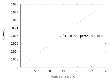
Figure 1
shows the evolution of the quantity ![]() according to time. It is by calculating the
slope of this line that we can obtain the diffusion coefficient D.
according to time. It is by calculating the
slope of this line that we can obtain the diffusion coefficient D.

Figure 1: ![]() according to time. The slope of this
line is the diffusion coefficient D.
according to time. The slope of this
line is the diffusion coefficient D.
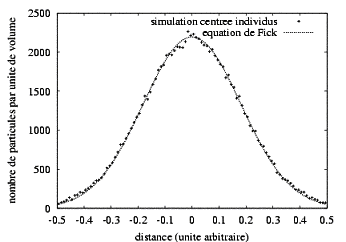
Then, one
can check that the microscopic model of the particles has the same behavior as
the macroscopic equation of Fick. Figure 2 makes it possible to compare the two
models.

Figure 2: Individual-based simulation for 105
particles (cross) and the equation of Fick (dotted line) with t=30s. The
simulation and the theoretical curve correspond almost perfectly. One regards
the two models as equivalents by their execution trace.
Figure 2
shows us the results of a simulation of the diffusion carried out with 105
particles for a 30 seconds simulated duration in a cube of 1cm3.
Speed is determined at random from a uniform law between 0 and vmax=0.1cm.s-1.
Equation 5 gives us the diffusion coefficient D = 5.10-4 s-2.
Individual-based simulation is adjusted very well with the equation of Fick. A
test of the c2
indicates that the two distributions are not significantly different: p(c2 =
24,76) > 0,5 with 30 degrees of freedom. This result is not surprising since we do
nothing but reproduce the experiment carried out in laboratory by physicist
J.B. Perrin and his students to measure the diffusion coefficient (Perrin,
1997). The first use that we thus make of multi-modeling within this framework
thus allows the determination of particular values of parameters or functions
of these parameters. The individual-based model is then regarded as a virtual
laboratory in which we conduce experiments on the system to determine
parameters of the aggregate model, here D. That we can thereafter
integrate into the differential equation (cf. equation 1) for an analytical
resolution.
4
Coupling
of the two models
In the
preceding paragraph and the former work applied to marine ecology (Duboz and
Al, 2001), we showed that it was possible to parameterize an analytical
equation using an individual-based model. We will show here that it is also
possible to parameterize a numerical scheme during its resolution. In the
majority of the cases, we do not have an expression of D according to vmax
which could be directly used in equation 2. We thus simulate the phenomenon
using the individual-based model to determine, for each iteration, and for each
section of the cube the value of Di. Which we reintroduce in
the equation of the numerical model for then determining by resolution of the
numerical model the values of the various concentrations in each section of
space (cf Figure 3). To identify each Di, we use the method
presented at the preceding paragraph, by using an individual-based model on 31
individuals only to limit the calculation time. We checked that the results are
equivalent to those obtained by simulating 105 individuals.
Even if
the conditions of simulation remain identical, the great stochasticity of the
individual-based model leads to variable values of Di in a
small interval. For the calculation of such a numerical scheme, it is thus
significant to know the field of variation of Di in order to
observe the conditions of stability.

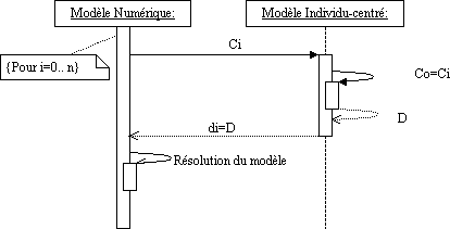
Figure
3: UML Sequence diagram for the illustration of the bi-directional coupling
between numerical model and individual-based model, for each section of space
i, the digital model will launch an individual-based model initialized with the
corresponding concentration to determine the coefficient of diffusion in the
section.
Figure 3 illustrates the coupling of
the two models. Such a coupling makes it possible to simulate the space effects
of the variation of the diffusion coefficient on the system dynamics. We will
illustrate this method by considering that the concentration of the particles
has an effect on their speed, for example by considering an escape reaction of
the ones compared to the others. This reaction to the concentration can be
modeled by a Monod type equation which makes increase speed according to the
concentration until a fixed maximum (equation 5).
![]() (equation 5)
(equation 5)
Where v is the speed of the
particles, vmax the maximum speed and c the concentration.
The model
is the same one as previously with for the expression the particles speed vmax
= 0.5 cm.s-1 and b = 10-3. We obtain the
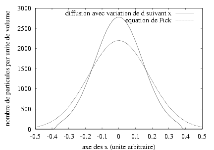
results illustrated by figure 4. The difference with the preceding case is that
the individual-based model at every moment needs the value of the local
concentration, which is given by the aggregate model. With such an assumption
of modeling, figure 4 shows that the particles do not reach the edge of the
cube for the same duration of simulation and that the bell form of the equation
of Fick is not preserved for the small concentrations. There is no question
here of making a precise study of this phenomenon but of illustrating the
coupling like a method of possible investigation.

Figure 4:
Simulation of the diffusion phenomenon during 30s by considering that the speed
of the particles decreases with the concentration (full line) by comparison
with the equation of Fick where speed is presumably constant (see the text for
the details).
5
Discussion
In the
two examples given previously (parameterization and coupling), we simulated the
same duration in the same space for the same concentration. However, the same
methods can be applied to different scales. In our toy example, the scaling
does not modify a priori dynamic thus the method is not of interest in this
precise case. We describe however how a scaling could take place, at only
illustrative ends. Let us consider the individual-based model simulating the
diffusion of a small number of particles in a small volume and, by using a
bi-directional coupling and the same assumptions that previously, one provides
to the integration scheme the value of the diffusion coefficient to each time
step, this last being higher than the time simulated by the individual-based
model and for each space step, larger than the cube simulated by the
individual-based model. Using a simple operator who makes shift the unit of the
diffusion coefficient to give it to the integration scheme, we simulate a scale
transfer.
This type
of coupling can be particularly interesting for the simulation of the animals
migrations for example, on a regional scale modeled using differential
equation, knowing that the individual behavior and the reactions to the
environment strongly influence the dynamics of the whole of the herd. The
individual-based model of "water balls" proposed by Servat (Servat
2000), could be the subject of a coupling with various aggregate models
(different according to the water quantity) usefully inspired of this approach.
One can suppose that it is also the case of many other applications. Since the
methods of Monte-Carlo, it is known that simulations having recourse to the
pseudo-random numbers can for example be used for the calculation of integrals
presenting limits of integration which are not easy to express analytically
(Press and Al, 1994). Simulation assists "here" mathematics, when
those reach their operational calculative limits. In the same way the methods
of numerical integration, although resulting from theorems and axioms shown
formally, were born from the need to solve numerically, i.e. by simulating
them, the generally analytically insoluble systems of differential equations. Our
approach is in the same line, by adding the idea of virtual experimentation on
the individuals-centered model.
We think
that this approach makes it possible in certain cases as well as possible to
use the advantages of the two types of modeling, and to obtain a real
appreciation compared to the use of only one of the models. Indeed, the
aggregate model makes it possible to obtain a compact and easily usable
representation of the whole of the model’s dynamics. The individual-based model
makes it possible to soften the use of the aggregate model by identifying its
parameters locally. One can in addition put the question of the effectiveness
of the on-line coupling. It is clear that in certain cases it can be more
advantageous to draw up a priori a protocol of tests in the virtual laboratory
and to draw from it the interesting values for the aggregate model. It is the
case in our example if the whole of the reachable values of vmax
are known a priori. Indeed, it is then enough to establish experiments for
various values of vmax in this interval, in order to obtain
by interpolation the function which gives D according to vmax.
This function is then directly used in the aggregate model. It is a generic
method to many other models.
6 References
Dautray
R. et Lions J.L., 1984. Analyse
mathématique et calcul numérique pour les sciences et les techniques.
Evolution : numérique, transport, vol 9, INSTN CEA, 1984.
Duboz R., Ramat E. et Preux P.,
“Towards a coupling of continuous and discrete formalism in ecological modelling:
influences of the choice of algorithms on results”, in proceedings of the ESS’01
conference, Marseille (France), p.481-487, 2001
Epstein, J. and Axtell, R., 1996. Growing
artificial societies, Social Science from the bottom-up, MIT
Press.
Ferber, J., 1995. Les systèmes Multi-agents, vers une intelligence collective.
Inter-editions, 1995.
Fick, A.,
1855. „Über diffusion“, Annalen der
Physik und Chemie, 94, p.59-86. 1855.
Fishwick P.,
1995. Simulation Model design and Execution. Building Digital
Worlds. Prentice Hall, 1995.
Forrest S.,
“Emergent computation : self organizing, collective, and cooperative
phenomena in natural and artificial networks, Introduction to the proceedings
of the ninth annual CNLS conference”, Physica D 42, p1-11, 1990.
Grimm, V., 1999.
“Ten years of individual-based modelling in ecology: what we have learned and
what could we learn in the future ?”, Ecological Modelling, 115, p.129-148, 1999.
Legay, J.-M.,
1997. L’expérience et le modèle, Un discours
sur la méthode. INRA
éditions, 1997.
Lindenberg, S., 1992. “The
method of decreasing abstraction.” In Rational choice theory: advocacy and
critique. T.Fararo (ed.), vol.7, Sage
publications, p.3-20, 1992.
Perrin, J.-B., 1997. L’ordre
du chaos. Bibliothèque Pour La Science, Pour La Science eds, 1997.
Press W. H., Teukolsky S. A., Vetterling W. T.,
Flannery B. P., Numerical Recipies in C,
(FORTRAN, PASCAL), The art of Scientific Computing, 2nd Ed,
Cambridge University Press, 1994.
Servat,
D. Modélisation de dynamique de flux par agents. Application aux processus de
ruissellement, infiltration et érosion. PhD Thesis
Paris VI, 162p, 2000.
Wooldridge, M. and Jennings, N.,
1995. “Intelligent Agents: Theory and Practice.”, The Knowledge Engineering
Review, 10(2), pp. 115-152, 1995.